Do you know how to harvest data from your bench tools, like plotting bandwidth from your oscilloscope with a computer? It’s actually pretty easy. Many bench tools make this easy using a standard protocol with USB to make the connection.
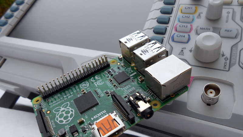
In the previous installment of this article we talked about the National Instruments VISA (Virtual Instrument Software Archetecture) standard for communicating with your instruments from a computer, and introduced its Python wrapper with a simple demonstration using a Raspberry Pi. We’ll now build on that modest start by describing a more useful application for a Raspberry Pi and a digital oscilloscope; we’ll plot the bandwidth of an RF filter. We’ll assume that you’ve read the previous installment and have both Python and the required libraries on your machine. In our case the computer is a Raspberry Pi and the instrument is a Rigol DS1054z, but similar techniques could be employed with other computers and instruments.
Our Real World Problem: A Low Pass Filter
A prototype low-pass filter for the 10m amateur radio band was designed using the QUCS simulator. The band sits at the top of the HF spectrum, from about 28 to 30 MHz, so the idea was to create a filter that lets everything below 30MHz through and attenuates everything above that frequency. The simulation showed a cut-off at 30MHz and a flat response for the upper 2 MHz of the passband. Almost perfect for the application.
But before celebrating it’s worth checking, does the filter really perform as well as its simulation? For that we need to measure its real-world performance, and to save the effort of repeated manual readings and calculations we’re going to automate the task using a Raspberry Pi.
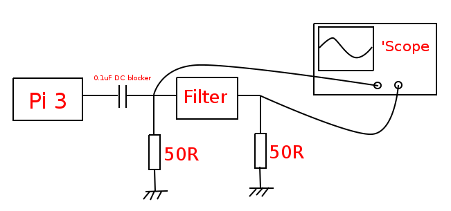
Our task is to measure input and output voltages for a range of RF frequencies covering the filter’s pass and stop bands, and to calculate the attenuation for each set of readings. As a source of our RF we’re going to use the Raspberry Pi’s on-board clock generator. This produces a logic-level output on pin 7 of the expansion connector which, after passing through a DC blocking capacitor, we’ll send to our filter.
Both input and output are taken into 50 ohm loads from which the ‘scope measures the RMS voltage. Our script then takes the two readings, and calculates a dB figure for the filter’s attenuation. It’s not the perfect measurement in that the input is not a sine wave, however once it has been through the DC blocking capacitor and faces the filter input at the terminator on the scope it’s a nasty rounded off waveform that for our purposes we can assume is an approximation to a sine wave without too much bother. We are interested in the shape of the curve rather than the absolute quality of the readings, so all that matters for us is that they are consistent.
Taking The Measurements
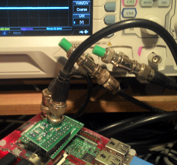
So our filter was mounted on our Raspberry Pi, and the ‘scope was hooked up with BNC leads, T-pieces, and terminators. The channels were enabled, what next? We already had Python and the required libraries from our previous excursion into Pi-scope communication, so it only remained to download and compile a copy of [Jan Panteltje]’s freq_pi signal generator.
This version has a mod to recognize more recent Pi processors, which the original lacked. Then the script below was created, and modified to reflect the path to the freq_pi executable and the Rigol’s resource name as described in the previous installment of this series. A better script might retrieve this last value from the ‘scope, but is beyond this demonstration. Specify start, end, and step frequencies in Hertz, and it will loop through each value and calculate a dB attenuation figure from the input and output readings for each one.
We saved our copy of the Python code as db-filter-analyser.py.
#!/usr/bin/env python
import time
import math
import subprocess
import visa
import matplotlib.pyplot as plt
#Start, end, and step frequencies in Hertz
startfreq = 25000000
endfreq = 32000000
freqstep = 100000
#The resource name for your 'scope, you'll need to change this line
resourcename = 'USB0::6833::1230::DS1ZA123456789::0::INSTR'
#Location of the freq_pi executable
freqgen = "/home/pi/freq_pi/freq_pi"
#Open the resource manager
rm = visa.ResourceManager('@py')
#Open the 'scope by name
oscilloscope = rm.open_resource(resourcename)
#Return its ID string to tell us it's there
print(oscilloscope.query('*IDN?'))
#Set up arrays, then loop
graphfreqs,graphdbs = [],[]
for freq in xrange(startfreq,endfreq,freqstep):
    print freq
    subprocess.call([freqgen, "-f", str(freq)]) #Call the RF generator
    #Read the input values from the 'scope and extract a float.
    #Input
    time.sleep(0.1) #Let everything catch up
    #Change CHAN to your channel number
    oscilloscope.query(':MEAS:SOUR:CHAN1')
    fullreading = oscilloscope.query(':MEAS:ITEM? VRMS,CHAN1')
    readinglines = fullreading.splitlines()
    inputreading = float(readinglines[0])
    #Output
    time.sleep(0.1) #Let everything catch up
    #Change CHAN to your channel number
    oscilloscope.query(':MEAS:SOUR:CHAN2')
    fullreading = oscilloscope.query(':MEAS:ITEM? VRMS,CHAN2')
    readinglines = fullreading.splitlines()
    outputreading = float(readinglines[0])
    #Calculate a dB value from the two readings
    decibels = 20*math.log10(outputreading/inputreading)
    print decibels
    #Add the values to the arrays
    graphfreqs.append(freq)
    graphdbs.append(decibels)
#Stop the RF
subprocess.call([freqgen, "-q"])
#Create our graph
plt.plot(graphfreqs,graphdbs)
plt.ylabel('dB')
plt.xlabel('Frequency')
plt.show()
Running the code requires sudo to use the USB port, for simplicity in this demonstration. If you are pursuing this you may want to allow your ‘scope to be used by non-root users by setting up udev rules for it. So meanwhile with the ‘scope turned on, connected, and with the respective channels enabled, we ran the script as follows:
sudo python db-filter-analyser.py
How Well Did It Match The Simulation?
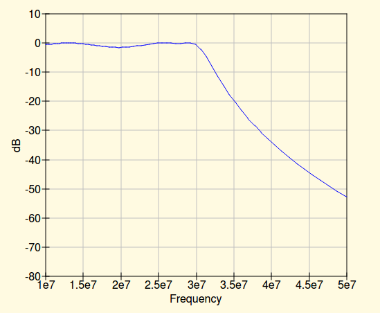
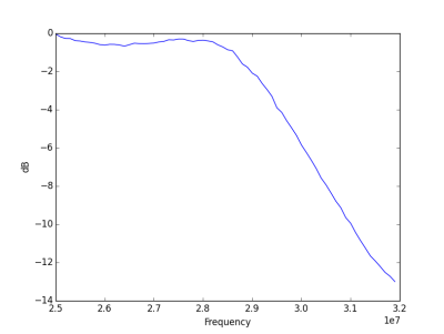 A list of dB readings from the filter scrolled up the screen, and eventually the graph appeared. So, how did our filter do? As you can see from the resulting plot on the left it exhibited a sharp cut-off, so it’s good at the job of being a low-pass filter. Unfortunately though it’s about a MHz too low, cutting off just below 29 MHz rather than the 30 we found in our simulation. Perhaps this is a function of component tolerances, or maybe just a misplaced trust in simulation. For this design at least it seems a return to the drawing board is in order.
The filter characterization shown here is not the most elegant way to perform the task, but it shows how it (and measurement problems like it) can be performed with the kind of equipment you have on your bench. You can control your instruments and take measurements from a computer — it’s no Dark Art — and you should have a go yourself with your own instruments and measurement problems. Whatever you do, be sure to share it with us on Hackaday.io!


Great stuff! Really shows how you can get extra value out of instruments you may already have with a simple script
The signal has (as you said: “nasty”) quite a bit of higher harmonics, which the low pass will attenuate more.
Could this translate into the perceived lowering of the filter cutoff?
By how much?
I wouldn’t think so, at least not when measuring that close to its cut-off. The first harmonic spike is still a long way away for a 30 MHz LPFwhen your sweep starts at 25ish MHz.
It’s designed for a Pi, so square waves are what it’s going to be fed in its working life, anyway.
I was thinking that as you probably measure the ratio of the averaged amplitudes (or powers?) before and after the filters, the higher harmonics get “pushed further down” the slope (well beyond the 30 MHz cutoff). But this should make the knee “rounder”, which we don’t see.
OTOH the higher harmonics are pretty far up, as you notice. The first relevant one should be the third (square wave), and would be 75 MHz for the start of your range (25 MHz). So your hunch looks much more plausible than mine :-)
Bench tool, huh? (http://welnz.com/products/measurement/bluetooth-caliper/)
I had a test at work where I had to read the frequency on a hall effect sensor every 10 minutes for 3 hours. I had to sit there and manually record the frequency and then convert it to RPMs. After reading this I wrote a simple python script to read the frequency, convert to RPM, and then output that a CSV file to import into Excel. Thanks for the great article and making my job easier.