What Every PCB Designer Needs To Know About Track Impedance With Eric Bogatin

September 12, 2022 by Dave Rowntree 7 Comments

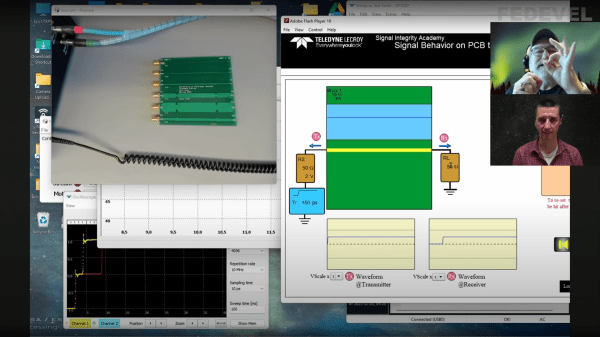
PCB design starts off being a relatively easy affair — you create a rectangular outline, assign some component footprints, run some traces, and dump out some Gerber files to send to the fab. Then as you get more experienced and begin trying harder circuits, dipping into switching power supplies, high speed digital and low noise analog, things get progressively more difficult; and we haven’t even talked about RF or microwave design yet, where things can get just plain weird from the uninitiated viewpoint. [Robert Feranec] is no stranger to such matters, and he’s teamed up with one of leading experts (and one of this scribe’s personal electronics heroes) in signal integrity matters, [Prof. Eric Bogatin] for a deep dive into the how and why of controlled impedance design.

RG58 cable construction. These usually are found in 50 Ω and less commonly these days 75Ω variants

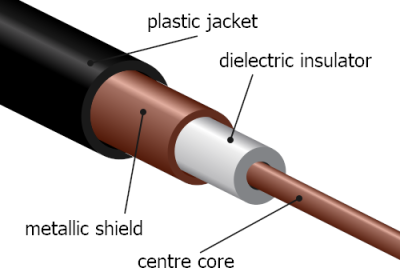
One interesting part of the discussion is why is 50 Ω so prevalent? The answer is firstly historical. Back in the 1930s, coaxial cables needed for radio applications, were designed to minimize transmission loss, using reasonable dimensions and polyethylene insulation, the impedance came out at 50 Ω. Secondarily, when designing PCB traces for a reasonable cost fab, there is a trade-off between power consumption and noise immunity.

As a rule of thumb, lowering the impedance increases noise immunity at the cost of more power consumption, and higher impedance goes the other way. You need to balance this with the resulting trace widths, separation and overall routing density you can tolerate.

Another fun story was when Intel were designing a high speed bus for graphical interfaces, and created a simulation of a typical bus structure and parameterized the physical constants, such as the trace line widths, dielectric thickness, via sizes and so on, that were viable with low-cost PCB fab houses. Then, using a Monte Carlo simulation to run 400,000 simulations, they located the sweet spot. Since the via design compatible with the cheap fab design rules resulted often in a via characteristic impedance that came out quite low, it was recommended to reduce the trace impedance from 100 Ω to 85 Ω differential, rather than try tweak the via geometry to bring it up to match the trace. Fun stuff!

We admit, the video is from the start of the year and very long, but for such important basic concepts in high speed digital design, we think it’s well worth your time. We certainly picked up a couple of useful titbits!

Now we’ve got the PCB construction nailed, why circle back and go check those cables?

Continue reading “What Every PCB Designer Needs To Know About Track Impedance With Eric Bogatin” →

Dead Simple Time-Domain Reflectometry With Just A Battery And An Oscilloscope

December 14, 2020 by Dan Maloney 29 Comments

“Time-domain reflectometry” sure sounds like something that needs racks of expensive equipment to accomplish. In reality, TDR is just measuring the time between injecting a pulse into a cable and receiving its echo, either from the other end of the cable or from some fault or defect along the way. It’s a useful technique, and as [Allen Wolke (W2AEW)] shows us, it can be accomplished with little more than a battery, a resistor, and an oscilloscope. And a little math, of course.

There are, of course, dedicated time-domain reflectometers, but all of them are really just elaborations of the basic principles [W2AEW] demonstrates with his simple setup. The oscilloscope is set up with a tee connector on one channel; one side of the tee is connected to the cable under test, while the shield conductor of the other side is connected to the negative terminal of a 9V battery. A resistor connected to the center conductor is used to complete the circuit, which sends a brief pulse down the test cable. The scope is set up to capture the outgoing pulse as well as the return pulse, allowing the time between the two to be measured. Some simple math gives the length of the cable, the distance to a fault, or with a little rearrangement, the velocity factor of the cable.

The video below shows the simple method at work on coax and Cat 5e Ethernet cable. It even worked on a roll of zip cable, which was a little surprising. If this technique is too simple, you can always elaborate a bit and roll your own TDR tester. Googly eyes optional, of course, but recommended.

Continue reading “Dead Simple Time-Domain Reflectometry With Just A Battery And An Oscilloscope” →

Recreating Fast Oscilloscopes Is A Slow Process

February 10, 2020 by Kristina Panos 20 Comments

If you want to do something you’ve never done before, there are two broadly-defined ways of approaching it: either you learn everything you can about it and try to do it right the first time, or you get in there and get your hands dirty, and work out the details along the way. There’s a lot to be said for living life by the seat of your pants. Just ask anyone who found inspiration in the 11th hour of a deadline, simply because they had no other choice.

Ted Yapo didn’t have a lot of high-speed design knowledge when he set out to build an open-source multi-GHz sampling oscilloscope, but he didn’t let that stop him. Fast forward a year or so, and Ted’s ready to build his third prototype armed with all the hands-on practical knowledge he’s gained from building the first two.

At the 2019 Hackaday Superconference, Ted gave a talk about his journey into the high-stakes world of high-speed design. It’s an inspiring talk, and Ted gives a good look into everything he’s learned in trying to build a sampling ‘scope. We think you’ll appreciate not only Ted’s work, but also the ease with which he explains it all.

Continue reading “Recreating Fast Oscilloscopes Is A Slow Process” →

Fast Video Covers Coax Velocity Factor

October 11, 2019 by Al Williams 14 Comments

We once saw an interview test for C programmers that showed a structure with a few integer, floating point, and pointer fields. The question: How big is this structure? The correct answer was either “It depends,” or “sizeof(struct x).” The same could be said of the question “What is the speed of light?” The flip answer is 186,282 miles per second, or 299,792,458 metres per second. However, a better answer is “It depends on what it is traveling in.” [KB9VBR] discusses how different transmission lines have different velocity factors and what that means when making RF measurements. A cable with a 0.6 velocity factor sees radio signals move at 60% of that 186,282 number.

This might seem like pedantry, but the velocity factor makes a difference because it changes the actual measurements of such things as dipole legs and coax stubs. The guys make a makeshift time domain reflectometer using a signal generator and an oscilloscope.

Continue reading “Fast Video Covers Coax Velocity Factor” →

Video: Putting High Speed PCB Design To The Test

January 24, 2019 by Bil Herd 48 Comments

Designing circuit boards for high speed applications requires special considerations. This you already know, but what exactly do you need to do differently from common board layout? Building on where I left off discussing impedance in 2 layer Printed Circuit Board (PCB) designs, I wanted to start talking about high speed design techniques as they relate to PCBs. This is the world of multi-layer PCBs and where the impedance of both the Power Delivery Network (PDN) and the integrity of the signals themselves (Signal Integrity or SI) become very important factors.

I put together a few board designs to test out different situations that affect high speed signals. You’ve likely heard of vias and traces laid out at right angles having an impact. But have you considered how the glass fabric weave in the board itself impacts a design? In this video I grabbed some of my fanciest test equipment and put these design assumptions to the test. Have a look and then join me after the break for more details on what went into this!

Continue reading “Video: Putting High Speed PCB Design To The Test” →

Poor Man’s Time Domain Reflectometer

April 15, 2016 by Al Williams 25 Comments

A time domain reflectometer, or TDR, is an essential piece of test gear when working on long cables. The idea is simple: send a pulse down the cable and listen for the reflection from the far end. The catch is that pesky universal constant, the speed of light.

The reason the speed of light is an issue is that, in a traditional system, the pulse needs to be complete before the reflection. Also, time is resolution, so a 1 GHz sampling rate provides a resolution of about 10 centimeters. [Krampmeier] has a different design. He sends variable length pulses and measures the overlap between the outgoing and reflected pulses. The approach allows a much simpler design compared to the traditional method.

Continue reading “Poor Man’s Time Domain Reflectometer” →

Hackers Measure Cable Lengths With Time Domain Reflectometers

July 27, 2015 by Nava Whiteford 12 Comments

[android] has built up a fast edge pulse generator for time domain reflectometry (TDR). TDR is a neat technique which lets you measure cable lengths using electrical signals and can also be used to locate faults within the cable.

TDR works by sending a pulse down the cable. When the pulse reaches the end of the unterminated cable it is reflected back to the source. By monitoring the delay between the original pulse and its reflection you can determine the length of the cable. We’ve seen projects that use TDR before, and it’s often used in telecoms industry to locate faults in long cable runs.

You can try TDR in your lab using only a scope to observe the delay and a function generator to create the pulse. However, the technique works a lot better with pulses that have very fast rise times. So [android] built a fast edge pulse generator based on [w2aew]s design. Then added googly eyes for good measure. His build works great and is a nice demonstration of the technique.