Despite what you may have heard elsewhere, science isn’t just reading [Neil deGrasse Tyson]’s Twitter account or an epistemology predicated on the non-existence of god. No, science requires much more work watching Cosmos, as evidenced by [Ast]’s adventures in analyzing data to measure the speed of sound with a microcontroller.
After [Ast] built a time to digital converter – basically an oversized stopwatch with microsecond resolution – he needed a project to show off what his TDC could do. The speed of sound seemed like a reasonable thing to measure, so [Ast] connected a pair of microphones and amplifiers to his gigantic stopwatch. After separating the microphones by a measured distance; [Ast] clapped his hands, recorded the time of flight for the sound between the two microphones, and repeated the test.
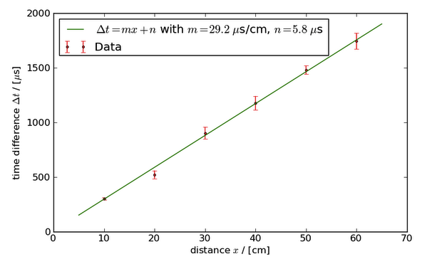
When the testing was finished, [Ast] had a set of data that recorded the time it took the sound of a hand clap to travel between each microphone. A simple linear regression (with some unit conversions), showed the speed of sound to be 345 +/- 25 meters per second, a 7% margin of error.
A 7% margin of error isn’t great, so [Ast] decided to bring out Numpy to analyze the data. In the first analysis, each data point was treated with equal weight, meaning an outlier in the data will create huge errors. By calculating the standard deviation of each distance measurement the error is reduced and the speed of sound becomes 331 +/- 14 m/s.
This result was better, but there were still a few extraneous data points. [Ast] chalked these up to echos and room vibrations and after careful consideration, threw these data points out. The final result? 343 +/- 9 meters per second, or an error of 2.6%.
A lot of work for something you can just look up on Wikipedia? Yeah, but that’s not science, is it?


I completely understand this urge to discover for yourself.
I’ve replicated a lot of fundamental constant experiments on my own, and I love it. The speed of light in vacuum and Cavendish’s torsion balance experiment for G have been my favorites so far.
It’s a wonderful feeling to sit down, think through an experiment, and end up measuring the weight of the world.
Nicely done, Ast!
Thanks. ^^
Agreed…
I participated as a citizen observer in an experiment that HAARP conducted several years ago. In that experiment, they beamed HF carrier pulses at the moon, and asked the public to listen for echoes.
There were two sessions. I recorded both of them with Audacity. Later, playing with the waveforms, I confirmed to myself that the echoes had indeed come from the moon by computing the distance the pulse had travelled based upon the delay time of the echo and the speed of light. Cool stuff.
I also used some of Audacity’s built-in analysis tools to demonstrate doppler shift in the echo as the moon swept past.
More post like this please
Sounds just like how all to many ‘scientists’ work now-a-days. Instead of doing the work required to improve the test setup and thereby get more accurate results, they will just manipulate their data to get better ‘correct’ results…
Have you read my article? There I point out that you DO NOT just manipulate your data to get the results you want if you want to do real science. Your aim is to get closer to the truth and whatever you decide to do with your data, you publish what you did, so others can decide for them selves whether or not that was justified.
I don’t know what ‘scientists’ you know, but the ones I know take their data seriously.
Also, this was an afternoon recreational endeavour and you have to consider the time-gain-trade-off. If I had to make a more accurate measurement that actually had any consequences aside from that number on my blog, I’d have put more time into reducing the errors in the measurement. ;)
Yes, as I said, manipulating data is very common now–anyone remember the phrase ‘hide the decline’… or perhaps the number of ‘scientists’ who have been discredited for manipulating their test data to ensure funding…
In science, outliers are not removed. All too often outliers serve to point to problems with either the theory (or in this case) the experimental setup.
Done properly, you would have adjusted the test environment to reduce/remove what you believed was causing the outliers and redone the tests…
That would have improved your results–if you were right about what was causing the outliers. But of course it was simply easier to manipulate the numbers…
If only you read the write-up you’ll see the justification for throwing out the outliers. It’s pretty obvious those data points that were circled were there because of some outside factors (echoes , room vibrations, the neighbour’s kids screaming etc.)
@Ast: I’m a bit confused of your remark that the offset doesn’t matter as long as it stays the same for all measurements. My memory’s a bit fuzzy about systematic errors, but let me explain my confusion through an example, say, because of parallax, sloppy placement or other kind of systematic errors the point you took as 10cm is actually, say, 15 cm from the source. Doesn’t that skew the result of your calculation? Now I was exaggerating the figure, my understanding was that if the systematic error is smaller than statistical error (for example ±0.5/sqrt(2) cm, since perhaps you were using a ruler with a 1 cm unit markers) then it doesn’t really matter. But anything larger than that should be taken into account. Last question, can the error of distance measurement be safely ignored for the error propagation calculation (something to do with error-in-variables model)? I never found a good rule of thumb for when it can be safely ignored or not (a relative error of less than x% is okay to ignore?) It’s been quite a while since I read GUM, so it might be that I had a couple of concepts wrong.
In general the systematic error does of course matter. And it’s not that easy to get rid of it, as I tried to show at the beginning of the article.
But if we take your example (measuring 15 cm instead of 10 cm for the first measurement), it actually makes no difference in this case, as long as the additional offset is the same for all data points. If we measure an additional 5 cm for every data point, the line will be shifted 5 cm to the right, but the slope will stay the same. And since we use only the slope to measure the speed of sound, that does not affect our measurement.
There are some other systematic errors that I ignored for the sake of not having to write another page and because they are much smaller than the accuracy I achieved:
1) The measuring tape might not be accurate, i.e. one cm on the tape is actually 0.999 cm. This is different from the constant offset as it would change the slope of the line and thus the speed of sound we measure!
2) My TDC might not be accurate, i.e. one of its seconds are actually 0.999 seconds. This, again, would change the slope of the line, but the effect is much smaller than the spread of the times I get because of statistical fluctuations.
In general, you ignore errors if they are much smaller than the other errors. It wouldn’t really make a difference whether you measure 123 +/- 6 or 123 +/- 6.003. On the contrary, quoting your error with a better accuracy than you actual value can be considered bad style. ;)
That is also the reason why I ignored the (pretty much statistical) error in the distance measurement. I always aligned the same point of the helping hand with a tic on the measuring tape. If you do this carefully, you get a quite precise positioning.
If the helping hand would have been positioned at random and I had to measure those random positions, you would be right and I would have to include the error on those measurements into the calculation.
Some years back, I wound up doing a much simpler version of this demonstration for a high school physics class. I arranged a pair of speakers separated by about thirty feet of phono extension cable and had a computer set up next to one of them play back and record a series of clicks. From there it was trivial to pull the time data off the recording, measure the difference between the distances from the computer, and average. Got pretty good accuracy, too- as I recall, it wound up being about 2% error as well.
That said, doing the same thing without using thirty feet of air is pretty damn cool.
Good example of how you need to treat every measurement as a pair of two values: the measured value, and the measurement error or accuracy.
In physics experiments at university, this was really drilled into us by the assistants. We had to do the regression calculations by hand, and every formula used to achieve a result had to be examined for the error propagation.
This is very well done here, and he does explain that cutting data after the analysis is cheating.
If he could increase accuracy to ±.5m/s, this would make a nice thermometer!
A cross-correlation between two microphones (even with just a hundred samples or so, depending on how much RAM the microcontroller has), would likely provide for a more accurate measurement because of the cross-correlation’s rejection of noise and echoes and so on. The microphones would likely need to be somewhat closer together, however. This is a pretty traditional method of performing ultrasound and seismological surveys but I think it would extend well to microcontrollers even with limited RAM. A parabolic fit to the cross-correlation peak provides resolution beyond the sample rate, as well.
The main problem I see here is the method for determining the transit time.
A more robust approach is cross correlation.
This requires recording 2 A/D channels
Pad w/ zeros to twice the length
FFT
Compute C = A x B* where B* is the complex conjugate of B.
The phase shift at each frequency is then 2*Pi*dT
Solve for dT by least squares.
The fundamental problem w/ using peak detection is that small differences in frequency response will move the peak. Room echos will also interfere more w/ peak detection.
An inverse FFT of C should show the peaks for each arrival and how the echo timing changes because of changes in source location. A couple of sticks (e.g. clava) will give a better source signature than clapping.
Sweeping an audio signal from 20-20Khz over a 10 s period will give even better results.
Have Fun!
I’m sure there are a few ways that would be better to accurately measure the speed of sound, but I needed a pretext to use my new TDC, so I opted for the traditional x/t approach. ;)
Oops. 2*Pi*f*dT
The edge of the text box gets cut off in my browser (Firefox 13.0) so it’s hard to proof read. A preview button would be nice.
Did you do a Q-test to see if you could throw out those pieces of data?
Once common approach is to compute the standard deviation and drop data outside 2 sigma.
A better alternative is to compute an L1 regression instead of the easier L2. glpk is very good for solving L1 (least sum absolute value). problems.
L2 is least sum squared error, so it’s more affected by outliers than L1.
I did not. And I have to admit that I had to look up what a Q-test is. As written in the article, I removed those points simply due to the fact that they looked quite far off from the others.
Not an approach I’d take for published research, but here it sufficed, I hope.
Of course, in the spirit of science you are welcome to check my procedures and apply the Q-test. ;)
Another fun way to do it is to use two speakers, play a sinewave through them and with a microphone measure the amplitude at different points between the speakers. Since you know the frequency of the tone, you can work out the wavelength from the interference pattern.
That DOES sound like fun. And it would also teach you something about waves.
Maybe as a first test for my signal generator and amplifier (works in progress)… ;)
Barring abnormalities, the final result seems a little bit high. Having not yet read the article I think there’s something that’s still off.
Using Excel, I’m unable to estimate errors. The linear trend-line function does not provide +/-errors, unless I missed something. I was able to follow just about everything else.
Otherwise, an interesting article.