Control systems are all around us, and understanding them is going to make you much better at hardware design. In the last article — Beyond Control: The Basics of Control Systems — we looked at an overview of what a control systems are in general with the example: “everything in between water and time is a control system”. We also observed control systems in nature, where I described my keen ability to fill a glass of water without catastrophic results. That discussion involved the basic concept of a block diagram (without maths) and we expanded that a bit to see what our satellite dish example would look like (still without maths).
I promised some big ugly maths in this article, and we’ll get to that in a bit, never you fear. First let’s have a look at how some basic elements: resistors, inductors, and capacitors are defined in the time domain. Don’t let these first few definitions turn you off. No matter how you feel about calculus, you don’t necessarily need to fully understand each equation. What’s more important is how the equations themselves combine to solve the circuit. Also important is that I will do everything possible to get out of doing difficult math. So stick with me through the article and you’ll learn that agony-saving trick for yourself!
A quick recap on transfer functions before we get going might be beneficial. A control system is used to define electromechanical behavior. For example: our satellite dish (from the previous article) at some point will need to be moved from one position to another position and as control engineers it is our job to determine just how this action will take place. I’m not talking about setting the mood for the big emotional robotic rotation, more like: not damaging the equipment or any people that might be nearby when moving the dish. For many reasons the dish would need to be moved with extreme care and in a very precise manner. The control system is the mathematical definition of that movement. Often the maths of the definition are nasty differential equations, (remember I’m avoiding any math that can be avoided, right?) so, instead of using differential equations to define the system, the transfer function will define the system with algebra, relating the output of the system to the input.
We aren’t going to be grinding out anything difficult but if you’re still worried about the calculus bits you should add [Will Sweatman]s Calculus is Not Hard series to your reading list.
Now let’s get familiar with some passive transients, shall we?
Defining Passive Components Mathematically
A resistor is an element that can be used to alter voltage and/or current, serving a variety of purposes that quickly become obvious and familiar when designing and building circuits. Although this is not an all encompassing definition for resistors it does allow us to communicate with the rest of the world what it is we’re using “that little one with the different colored stripes” for in our circuits.
If we wanted to explain this to someone with a mathematical background then we need to alter this definition so that it would be useful to them. For resistors this is not a problem, get really close to the mic and in a deep voice say “Ohm’s Law” while making eye contact (mean mugging the kids are calling it), drop the mic and walk out.
In the case that you forgot, Ohms Law states:

That is voltage is equal to the product of current and resistance.
Defining energy storing elements is not quite as simple. Transients require a little bit of fancy footwork and a careful exit strategy to keep from stepping on our own tongue while getting out of the room alive.
Lets have a look at how each element is analytically defined in terms of voltage and current in the time domain:
Resistor


I have included the symbol for a resistor that should suit you no matter which side of the pond you reside on. The calculations we use for resistors are the very essence of Ohm’s Law: V=IR or voltage is equal to the product of current and resistance. Fair enough, although it doesn’t seem that spectacular the first 600 times you use it, at some point you start getting creative with Ohm’s Law and it comes in handier than a spare $20 in your shoe. For our purposes we can think of the value a resistor represents as a constant, if you aren’t up to snuff on your calculus: constants = easy like Sunday morning.
Inductor


This isn’t quite as easy to explain to someone without a little calculus under their belt. For the most part if your response to those equations is something like “right, that’s bananas. I don’t like it, and I won’t stand for it.” then we’ll be okay. At this point in our controls discussion we aren’t required to work through any calculus. Believe you me, I don’t want to explain it any more than you want me to. The point of including the calculus equations is to remind those of us who haven’t had to work through a derivative (that’s the one on the left with 2 many d‘s) or an integral (the one on the right with big stupid ∫ with numbers on the wrong ends of it) in a while just how much we don’t remember the mechanics of it.
Capacitor


A good eye will spot the similarities in the capacitor and inductor equations.
Time Domain Analysis
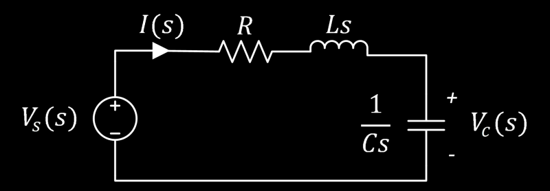
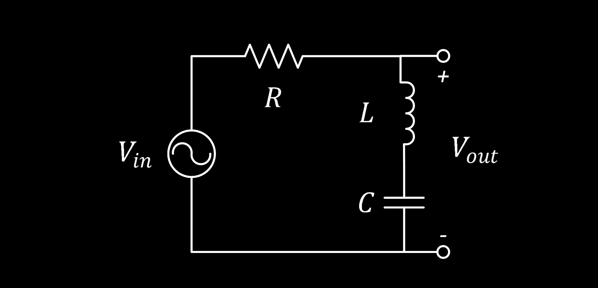
You can see how things can get mathematically hairy if we have a few capacitors (C) and inductors (L) in a circuit that needs to be defined analytically. Just to drive the point home, have a look at a basic series RLC circuit (I’m assuming you can make the leap of faith as to what the R represents).
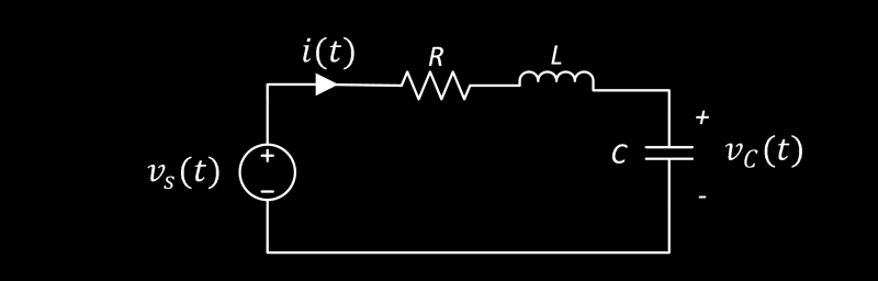
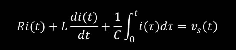
The series RLC circuit shown above can be modeled using the time domain definitions that we previously discussed. The voltage equation for each component is what goes into the right side of the equation. When you get all the bits together it’s basically an intimidating version of Ohms Law, as you can see below.
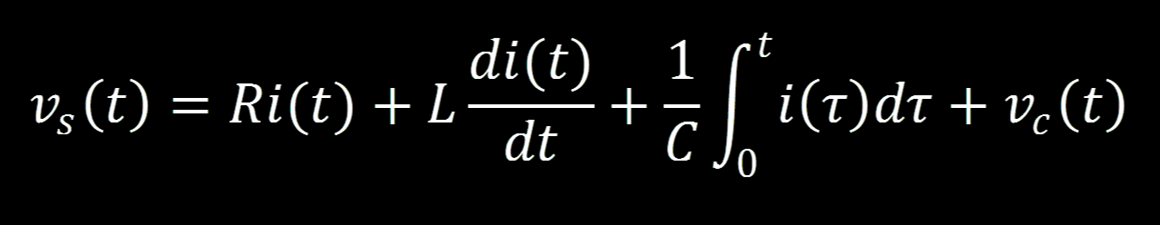
If you’re breaking into a cold sweat as a result of that equation take a deep breath, step back, and let’s talk about this. I said it was going to be a big hairy Ohm’s Law equation remember? Take a look at the term on the left side of the equation and the first term on the right side and cover the rest with your hand, now ignore the (t) in both terms and what do we have? You got it, V=IR and the following terms are the definitions of voltage for each component. Adding the voltage of each component together results in the total voltage in the circuit for any time t (aka: voltage as a function of time). The symbol tau used in the capacitor term of the equation is a time constant as well. We won’t get into how to find tau at the moment but I just told you this equation is a function of time and didn’t want you calling me out on tau.
In order to evaluate this equation lets get rid of the integral by taking the derivative of the entire equation, leaving us with a 2nd order differential equation. I realize that you weren’t warned about the differential equations but just hold on a sec before you run to the comments to taddle, it’ll be quick like a Band-Aid.
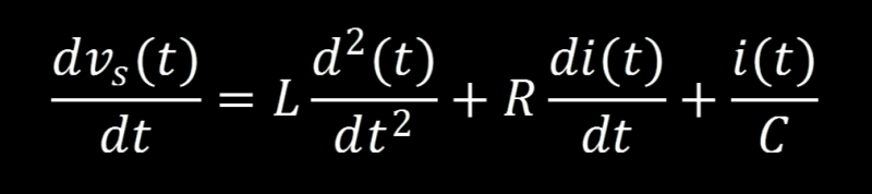
A differential equation (DFQ) can be solved in the time domain but look at that monster we’ve created, it must be a joke, right? Also keep in mind that we haven’t replaced the RLC variables with the component values, this has the potential to get horrific. Replacing L with 20E-6 won’t make the arithmetic any different, it will however cause it to look even more intimidating and most importantly: when I have to keep track of numbers on paper rather than symbols, mistakes will be made. Conclusion: lets attack in another direction.
S-Domain = Algebra instead of Differential Equations
As you can see from the differential equation we decided to steer clear of, this is complicated. To simplify things we can handle these nasty time domain equations in the s-domain. It might be easier to wrap your head around this concept if you think of the s-domain as the complex frequency domain. This allows us to solve complex calculus equations using algebra. But how can this be? Why would calculus be a thing if we can just algebra our way out of it? That’s a great question: because Laplace. The Laplace Transform is how we get from the time domain to the s-domain. Not surprisingly we use the Inverse Laplace Transform to return to the time domain when we’re done messing about in the s-domain.
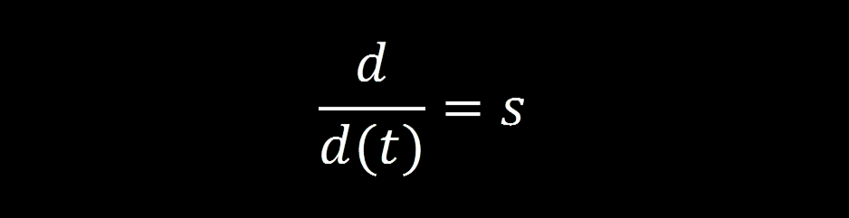
The s-domain equivalent of a derivative is the complex variable s. Remember this substitution and things will start to make sense as we go from one domain to the other.
Laplace Transform
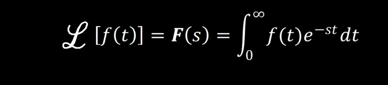
The general form of the Laplace Transform can be seen above and if you desire it can be used as described. We aren’t going to need it in this article but it will come up again in a subsequent article when we go from the s-domain to the time domain. So here it is in all its glory for you to refer back to at a later date, but for now, we should keep moving.
Passives S-Domain equivalents
The s-domain will allow us to replace calculus with algebra. This can be done not by magic, but careful redefinition of our mathematical statements, expressions, and equations. Resistance in the time domain is equivalent to impedance (Z) in the s-domain so our Ohm’s Law equation in the s-domain is:
Below you will find the s-domain equivalent impedance for each component. Derive them on your own if you wish, this article is already mathy enough for me without anymore proofs.
Resistor s-domain Impedance
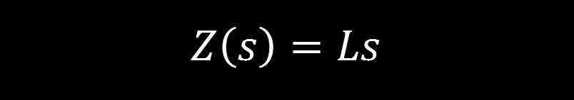
Inductor s-domain Impedance
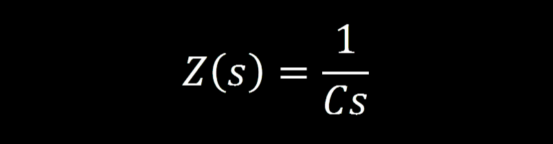
Capacitor s-domain Impedance
Control Systems, was it?
Meanwhile, back to the point: I bet you thought I forgot what we were even doing here? You’re right, I got all caught up in multi-domain definitions of circuit elements but don’t touch that dial because I’m about to shoe-horn some controls in here. Lets see how (if at all) this relates to a control system.
Lets find the Transfer Function relating the capacitor voltage to the supply voltage using the original RLC circuit.
We’ll step through the process of each approach, the DFQ and transform.
Differential Equation with Mesh Analysis
Starting with the resistor and working our way around the loop in a clockwise rotation we have:
Using the relationship between current and charge:
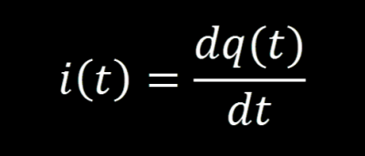
We can substitute out every i in the equation. This results in a 2nd order DFQ:
We of course remember that the charge of a capacitor is equal to the product of the voltage across the capacitor and its capacitance:
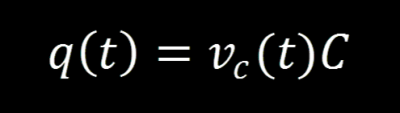
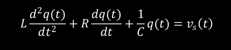
We use the relationship to replace the charge q:
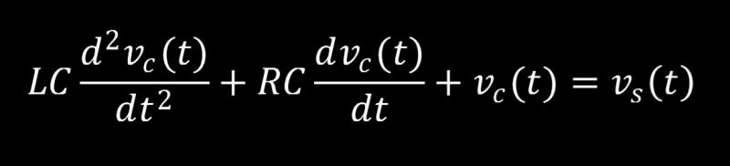
Take step back to observe the beautiful differential equation we have constructed, this is an emotional moment we’re sharing right now. Dry your eyes and lets move from the time domain to the s-domain by using the Laplace Transform. By substituting the complex variable s for the derivatives and factoring out the voltage across the cap (Vc(s)) we have a much cleaner equation:
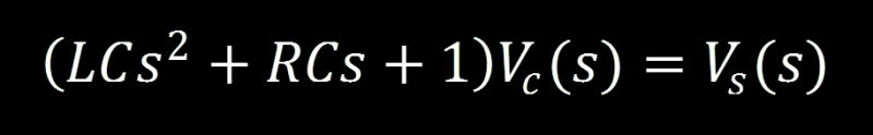
Finally, we can solve the equation for the ratio of output to input for our control system, resulting in the transfer function:
Transform Method with Mesh Analysis
If we redraw our circuit with s-domain equivalent impedances before creating the loop equation we have this circuit:
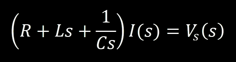
Now we write our loop equation the same way we have each time when looking at the schematic:
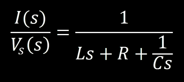
Solve for current over voltage:
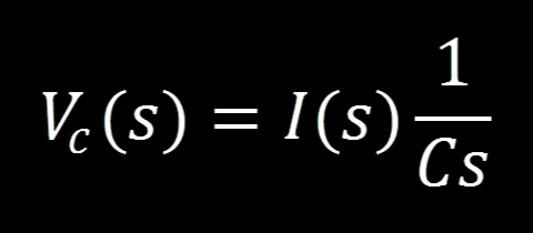
Using the impedance equivalent of Ohms Law for our capacitor voltage:
We can solve for current and use the result to replace the current in our “current over voltage” equation:
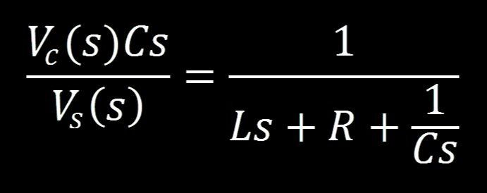
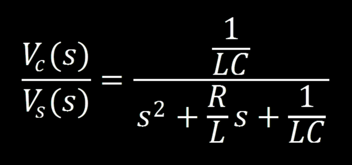
We can solve the equation for the ratio of output to input for our control system, resulting in the transfer function:
Why did we arrive at the same equation twice?
I really hope this is rhetorical because it is SO exciting that this happened! I mean we TOTALLY avoided solving a 2nd order differential equation! We just blasted right thru the defense with nothing but algebra, made a few crossovers, one behind the back pass and straight dunked a transfer function like a boss! I don’t play baseball but that sounds like an easy win to me.
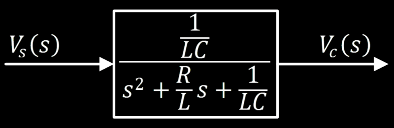
Resulting Transfer Function
We know that the transfer function is the mathematical representation of the control system, so we can take our transfer function and put it in the block diagram of the control system:
What does it all mean?
The fact that this is very technical is not lost on me, so maybe I can shed some light by trying to bring this full circle: We can design an RLC circuit to be a notch filter for an AC signal, which is also known as a band-stop filter. This is useful for a variety of applications such as blocking pesky 60Hz noise. One way we can do this is by taking the output of our circuit across the inductor and capacitor, like so:
This is useful for blocking only part of an input signal. However we aren’t blocking in the form of clipping the signal, which would be blocking any voltage over a specified value. We are blocking parts of the signal which are defined by a range of frequencies, in this case it would be the “stop band”. We can define this range of undesirable frequencies by choosing inductor and capacitor values which create resonance at the center of the desired stop-band. I think we should forego any further maths for now as I’ve had my fill and I think you’re picking up what I’m putting down at this point.
Conclusion
We covered how to create a transfer function from a simple RLC circuit. We defined passive elements in multiple domains. We used those definitions to find a simple RLC circuits transfer function. In the next installment of Beyond Control I plan to discus how we can find the time response from a transfer function and what some of its characteristics look like. We will also look at poles and zeros as a way to determine how a system will respond to various inputs and then I’ll then explain what poles and zeros are, cheers!


Nothing like a dose of circuit math on a Xmas eve to bring back memories of decompressing after end of semester exams in which these sorts of calculations figured strongly many years ago.
Hennessey Black and its all all good
OMG you’re worst than wikipedia.
“This isn’t quite as easy to explain to someone without a little calculus under their belt.”
WTF you dont need calculus to understand electronic… complexe number are actually more useful…
All equations for electrical circuits are derived from Maxwell’s equations by applying various calculus and differential equation techniques. Those complex numbers that you say are “more useful [than calculus]” are actually the solution to differential equations. You can design many electrical circuits with only algebra (as I do at my hardware design job), but anything more complicated (e.g. RF filters) requires calculus tools to design.
Sure, but Maxwells equations were a “unified” set of disparate equations for static fields. Ohms law falls out of Maxwells equations, but the former came first. You can do the majority of RF filter design with zero calculus, hence the compendiums of filter tables and equivalent circuits such as the MYJ book.
I think you mean “can be derived from”… Ohm published his work including Ohm’s law 4 years before Maxwell was born…
That was just a sneaky ploy so he could claim later that he wasn’t influenced by Maxwell…
I always found it more intuitive to view plots of those equations. I still imagine the plots when I’m thinking about what I need a circuit to do or how a circuit works.
I guess I should add that when learning filters we were asked to “reason out” the filter type by the placement and type of components present, and then check that reasoning by doing the math. It falls back to imagining what each component does and how that affects the value of voltage or current over time.
Letting the machine overlords have their fun would be a next step:
http://www.nutonian.com/products/eureqa/
Tutorial articles are usually welcomed, but meaningless text between equations won’t help too much, no matter how good or bad is the reader’s skills. For the next article, please try to make the math and the text sustaining each other.
To solve a 2nd order differential equation, you assume that the solution is an exponential. You do that because every other time you had a 2nd order DE the answer turned out to be an exponential.
You don’t know what the parameters of the exponential are yet, so you use letters for those. Substituting Ae^Bx into the DE, you can then take the differential of the exponentials you just substituted in, and the result is an ordinary equation with exponentials and no differentials.
When you do that, the original exponential will appear in all the terms, so it can be divided out across the board. You are left with the original factors, and the exponents from differentiating the exponentials once or twice.
The result is a 2nd degree polynomial which can be solved for the function that appeared in the original equation.
You still have a couple of A’s and B’s in your solution left over from when you substituted the exponential “guess”, so you look to your initial values. Usually you know the initial values at T=0 or T=infinity or some other known values, so you can substitute those in and solve for A and B.
Laplace noticed this trend – of substituting an exponential and then factoring it out again – and came up with a shortcut that eliminates the exponential step. You go directly from the differential to the polynomial, and then back again.
Differentiating an exponential results in xe^x, and this is a common form, so the Laplace transform is sF(s). You can eliminate the middleman by just writing down a table of commonly encountered terms, and what the results would be if you had done the exponential step.
That’s what the Laplace transform does.
For the readers who are afraid for the math belonging for PID control I can recommend a very old book written by Thompson, Silvanus P. (Silvanus Phillips), 1851-1916
Calculus Made Easy
Being a very-simplest introduction to those beautiful methods which are generally called by the terrifying names of the Differential Calculus and the Integral Calculus
Download it for free.
http://www.gutenberg.org/ebooks/33283
This was very well written and explains the subject as well as you will find anywhere. Thanks..
Emailing links to fellow enthusiasts now..
In the complex laplace domain:
Multiply by “s” -> you integrate
Divide by “s” -> you differentiate
In the real domain:
Differentiate then integrate a function (by the same differential operand dt) and you get the function back again because differentiation is the inversion of the integration.
In the complex laplace domain back again:
Multiply 1/s and s – the “s” is canceled out and you get a “1” because it’s algebra and s^-1 is the inverse of s.
2nd order in Laplace domain:
Divide by “s” square (1/s^2) -> differentiate two times (= 2nd order)
Ahh laplace-transformation I love it.
correction:
exchange “integrate” by “differentiate” and vice versa .. sorry.
So, just a thought. If you really want to start with basics, maybe remind the lay readers what actually is happening to current and voltage in inductors and capacitors; that is, why the calculus indicates changes in current or voltage cause a change in the corresponding quantity. That may help tie the math with the observed results in real circuits.
Of course, at the risk of spoiling all this, why not just refer to a classic text or any of several online; first I found has the information above in Chapter 3 http://www.ece.rice.edu/~dhj/courses/elec241/col10040.pdf
My last comment is that there is an assumption that everyone will approach control theory from an electrical perspective. As common and important is the mechanical aspect. Why not explain things in terms of the classic Mechanical Engineering springs and dashpots/shock absorber analogies?
I think that the electrical approach is often used for two reasons. First, in many programs only the electrical engineers cover control systems in any great depth (it’s often just skimmed in mechanical undergraduate programs), so many of the examples out there just happen to be electrical. Second, electricity is an inherently mathematical subject because you need something (math) to explain/model the stuff you can’t see! I’ve heard many times that Watt invented the fly-ball governor that we see on his steam engines, but was not able to explain rigorously how it worked (someone else did that later). You can understand it intuitively as he did without math, like most simple (and mean just the simple ones!) mechanical systems since we can see the parts.
I agree, though. The 2nd order equation of motion is just as good (and a mechanical analog of) the RLC circuit
In your first equation in the “time domain analysis” section you have vc(t) twice. Once as the integral and once as the symbol “vc(t)”. You should delete the last term.
Agreed, was just reading the comments to see if anyone else spotted this.
What I don’t fully understand is why, in this equation https://hackaday.com/wp-content/uploads/2015/12/time_madness_01_boxy.png
voltage of the capacitor seems to be represented by two terms of the equation : the integral term PLUS Vc. I understand that Vc is the voltage output of the circuit, but I’m not sure to understand how it gets its place here…
He made an error – see Chris’s comment above.
HORRIBLE MISTAKE
In the integrals, the limit should be from 0 to t, not 0 to 1. 0 to 1 makes no sense.
Your integrals are all taken from 1 to t, but are integrals of functions with respect to Tau. I think that’s a mistake, and that the integrals should be of functions with respect to ‘t’ (time). Assuming ideal conditions, Tau doesn’t change for a circuit, whereas ‘t’ does. There’s no point in integrating or differentiating with respect to a constant…the result is either ‘0’ or the result of multiplication.
The integrals should be from 0 to t, in which case the tau is required as you can’t take an integral of a function of t, to the boundary t. It’s a common substitution.
Excellent.
I think the exciting part of this is that with Laplace transforms (and other kinds of transforms), we can change a calculus problem into an algebra problem, and maybe even into a graphical problem. Root-locus analysis comes to mind.
Just wanted to say thanks to Brandon for tackling a topic that fills a shelf or two of my home bookcase. Thanks again.