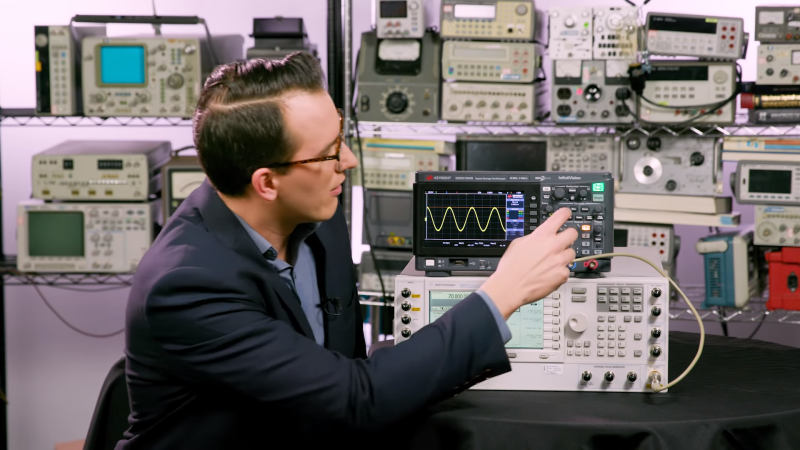
Oscilloscope bandwidth is a tricky thing. A 100 MHz scope will have a defined attenuation (70%) of a 100 MHz sine wave. That’s not really the whole picture, though, because we aren’t always measuring sine waves. A 100 MHz square wave, for example, will have sine wave components at 100 MHz, 300 MHz, and the other odd harmonics. However, it isn’t that a 100 MHz scope won’t show you something at a higher frequency — it just doesn’t get the y-axis right. [Daniel Bogdanoff] from Keysight decided to think outside of the box and made a video about using scopes beyond their bandwidth specification. You can see that video, below.
[Daniel] calls this a “spec hacks” but they aren’t really hacks to the scope. They are just methods that don’t care about the scope’s rated bandwidth. In this particular spec hack, he shows how the frequency counter using a 70 MHz scope’s trigger circuit can actually read up to 410 MHz. A 100 MHz scope was able to read almost 530 MHz.
It is interesting that the frequency counter works from the scope’s trigger circuitry which has its own signal path and isn’t going through the analog to digital converter. Of course, your scope might also have a frequency measurement function that reads the trace on the screen. That would probably work too, because you don’t really care how much the signal is attenuated just to read the frequency. Regardless, this is a neat trick to have in your bag.
Honestly, we are surprised the scope makers don’t characterize and rate this as part of the spec. We are pretty sure garden variety probes on a 70 MHz scope aren’t behaving as promised at 400 MHz, so maybe that’s part of the reason why they don’t.
If you have some spare cash, you could just get a 110 GHz oscilloscope, which ought to be enough for anyone. Of course, there’s more to a scope than just its bandwidth, but if you want to learn more about testing bandwidths, we’ve done that on some scopes both new and old.


I kinda don’t understand the point of the video: Look at the output of the signal generator! It’s 410 MHz, sure… at +25 dBm! It’s freaking *huge* – that’s *11 V* peak to peak voltage. The scope could have 60 dB of attenuation and you’d still have a 10 mV peak to peak signal.
I mean, the native “frequency limit” of the acquisition path is Nyquist, or 1 GHz, since it’s a 2 GSa/s scope. Anything below that and if you shove enough power at the thing and you’ll see *something*, and if you do an FFT of it, the majority of the power’s still probably going to be at the fundamental frequency. And while the trigger path probably does have less attenuation than the acquisition path, just seeing “what’s the highest frequency I can get on the frequency counter” doesn’t really tell you how useful it is.
This guy appear to get it.
Appears*
Yes and no. It’s obviously not making the scope a better scope, it’s pointing out a function that’s always been there, which most of us probably never realized was there. I certainly had no idea the frequency counter didn’t just count the traces on screen.
I’m gonna try to test this soon, since I have access to a 1.5GHz scope and a 2.7GHz signal generator, but the standard probes only go to 700MHz. See where the limits are…
I 100% agree with a lot of what you are saying. It was really more of a “because it’s there” type challenge for me. I wouldn’t recommend debugging with this approach, but I did find it interesting to be able to go this high in frequency.
The example was kind of trivial, but there’s a more basic idea that’s legitimately useful:
As he says at the beginning, we usually think about using a scope to capture an accurate representation of the signal of interest. The scope doesn’t stop working when you apply a signal higher than its bandwidth though. You just stop seeing an accurate representation of the signal. Instead, you see a representation that’s distorted by the scope’s bandwidth limits.
Those limits are well defined though, and you can extrapolate the actual input from the distorted output if you know how.
A slightly less trivial example would be measuring pulses faster than the scope’s native resolution.. let’s say a 100ps-to-1ns pulse going into a 100MHz scope. Obviously you won’t see crisp rising and falling edges, but the peak voltage of the curve on the screen will be a function of the scope’s impulse response, the amplitude of the pulse, and the width of the pulse.
Assuming you know the amplitude of the pulse and the scope’s bandwidth is exactly 100MHz, the pulse width will be 10.5ns x Vpeak / Vpulse to within about 0.1% error. That’s not bad for signals 10x to 100x faster than people would normally expect the scope to handle.
77mph??????
Everyone knows it’s 88!!!!
Right?! How can you trust someone on being right at something when he makes a mistake like this? 5 second googling would have revealed that for him. And it’s on the official Keysight channel.
That was the joke!
There’s a reason that a multi-GHz frequency counter is much cheaper than an oscilloscope.
Totally!
Thanks for the post, Al! We definitely don’t spec things like this, but we do often have info around the frequency response of a scope if someone asks for it. As you probably know there’s some nuance around gaussian vs. brickwall responses.