Spice is a circuit simulator that you should have in your toolbox. While a simulator can’t tell you everything, it will often give you valuable insight into the way your circuit behaves, before you’ve even built it. In the first installment of this three-part series, I looked at LTSpice and did a quick video walkthrough of a DC circuit. This time, I want to examine two other parts of Spice: parameter sweeps and AC circuits. So let’s get to it.

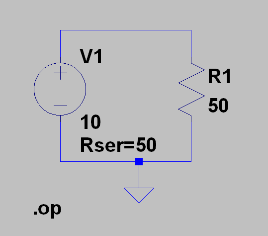In the first installment, I left you with a cliffhanger. Namely the question of maximum power transfer using this simple circuit. If you run the .op simulation you’ll get this result:

--- Operating Point ---
V(n001): 5 voltage
I(R1): 0.1 device_current
I(V1): -0.1 device_current

The power in R1 (voltage times current) is .5 W or 500 mW if you prefer. You probably know that the maximum power in a load occurs when the load resistor is the same as the source resistance. The Rser parameter sets the voltage source’s internal resistance. You could also have created a new resistor in series with V1 and set it explicitly.

If you think that this example is too simple to be of value, remember that a power source and a series resistor makes up a Thévenin source, and you can convert any linear circuit into its Thevénin equivalent and model it like this. For now, suffice it to say that V1 with 50 ohms of series resistance could stand in for a radio transmitter or some other complex device where you know the output impedance.

The reason that matching the resistors causes the most power to flow is because the source resistance forms a voltage divider with the load resistor. Here’s some handwaving to motivate the result. If R1 were completely open, the voltage at the top of R1 would be 10V, but with absolutely no current flowing. That’s zero watts of power. If R1 were a short, infinite current would flow, but with R1 nothing more than a piece of wire you’d have 0V across it and, again, no power.

When R1 is equal to the source resistor, you get a 50% voltage divider. That means R1 will see 5V and the current will be 10/100 = 0.1. This matches the results from Spice. But it doesn’t give you a good feel for why that’s the best. Clearly, lowering R1 would increase current right? Why does passing less current yield more power?

One Step at a Time

To answer that question with a thousand-word picture, we need to add a .STEP command to the schematic. On the LTSpice toolbar, there is an icon that reads .op. You can also press S or select Spice Directive from the Edit menu. Use that to enter the following:

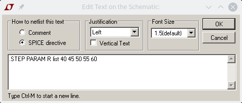
Then change the value of R1 from 50 to {R}. That looks strange, but the braces tell Spice this is a parameter, and the R matches the R in the directive. Because of the keyword list, Spice will now run the simulation with R=40, 45, 50, 55, and 60 ohms. Here’s a plot of the voltage, current, and power through R1:

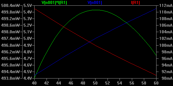
The green plot is the power, the blue is voltage, and the red is current. While the current does go up as the resistance goes down, the voltage drops which results in the lower power. Conversely, higher voltages result in lower currents. The 50-ohm spot is just right.

If you don’t want to walk through a list, you can omit the list keyword and use a command like:

.STEP PARAM R 40 60 5

This gives the same result because it sweeps R from 40 to 60 in steps of 5. You can get the same result by using the .DC analysis instead of .OP, although it isn’t very obvious. If you right-click on the .OP text on the schematic you can select DC sweep from the resulting dialog. The help text implies it sweeps voltage sources (which is true). However, for the source, you can enter PARAM R and then you don’t need the .STEP directive at all.

The resulting line should read:

.DC LIN PARAM R 40 60 5

The LIN part of that command tells Spice to step the value in a linear fashion (that is, 40, 45, 50). That’s the default. However, the .DC and .STEP commands let you specify OCT for octave or DEC for decade sweeps.

With the .OP or .DC command, the output fills in the blanks (in other words, you can read values for 42 and 44 ohm). However, for other simulation types, you will get discrete output for each step. For example, try changing the .OP command to a .TRANS command. The output will be correct, but it is hard to determine which group of plots go with which value of R in that case.

A Real Pane

One way to solve that problem is to create multiple plot panes using the Plot Settings menu. This lets you plot multiple things on separate graphs. On the same menu, there is a selection that allows you to pick which steps you want to display for a particular pane. Just be sure to uncheck the “apply to all panes” button.

There are many things you can do with panes and plots. For example, you can drag a label from one pane to another to move that waveform to the new pane. Using the Control or Alt key while clicking a label is usually interesting (although under Wine, the Alt key probably won’t work as expected).

Another trick is to drag a box on a plot with your mouse. Before you let go, you can read statistics about the selection at the bottom left side of the LTSpice window. Of course, when you let go the plot will zoom, but you can always undo (F9) to go back to the original view.

Even without panes, the step selector lets you look at one step at a time instead of all of them merged. However, for a .DC or .OP analysis, the plot works out fine with no extra steps.

An AC Circuit

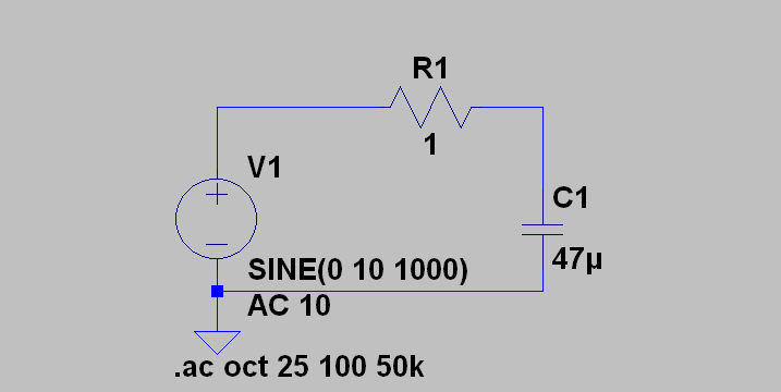Consider the circuit on the right. It has a few new things. First, the voltage source has an AC amplitude of 10 V (used in the .AC analysis) and it also is a sine wave of 10 V at 1000 Hz (utilized in the .TRANS analysis). There’s also a capacitor. Even though the schematic shows the Greek mu character for micro (as in 47 microfarads), you enter it as a “u.” You don’t need to find the code to enter the mu on your keyboard.

The .AC analysis sweeps the frequency of the source, in this case from 100 Hz to 50 kHz. The number of points per octave is 25. Here’s the output of the analysis (measured at the junction of R1 and C1):

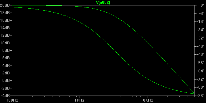
As you might have guessed, this is a crude low pass filter. Frequencies below 1 kHz pas through pretty well, but signals above that get reduced as C1 shunts them to ground. The bottom line is dashed (hard to see on the screen shot) and represents the phase of the signal (note the right-hand vertical scale). If you don’t want to plot the phase, click on the right hand scale and you’ll see an option to not plot phase angle.

Another way to represent this is using the .TRANS analysis and a .STEP command. To see this, change V1 to have a frequency of {F} and then add the following directive:

 .STEP PARAM F LIST 1K 10k 100k

Finally, replace the .AC simulation directive with .TRANS .005. If you plot the output (that is, the voltage between R1 and C1):

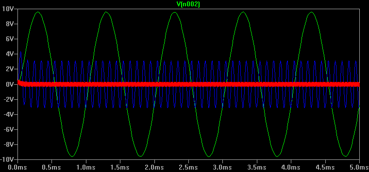
Here it is easy to tell the green trace is the 1 kHz signal, the blue is the 10 kHz, and the red is the 100 kHz. Note the differences in amplitude.

Theory vs. Practice

The only problem with the above simulation is that it is wrong. Real components don’t act like the perfect parts we used. The voltage source has some internal resistance. Capacitors have some resistance. Resistors have some reactance. Even wires aren’t perfect conductors.

Depending on what you want to accomplish, some of this may not matter. Next time I’ll talk about what happens to our filter circuit when real world components come into play. Meanwhile, here’s a question: What happens if you change the filter schematic so that C1 is where R1 is and R1 goes in the place of C1? Why not try it and see? Remember, using Control+R while dragging a component will rotate it. You’d probably want to use the open hand dragging when you try this.