If you want to simulate a tic-tac-toe game, that’s easy. You can evaluate every possible move in a reasonable amount of time. Simulating antennas, however, is much harder. [Rosrislav] has been experimenting with using simulated annealing to iterate antenna designs, and he shares his progress in a recent blog post.
For many problems, it simply isn’t possible to try all possible inputs to determine what provides the “best” result. Instead of trying every single input or set of inputs, you can try random ones and discard all but the best guesses. Then you make small changes and try again. The only problem is that the algorithm may lock in on a “local maximum” — that is, a relatively high value that isn’t the highest because it forms a peak that isn’t the highest peak. Or, if you are looking for a minimum, you may lock on to a local minimum — same thing.
To combat that, simulated annealing works like annealing a metal. The simulation employs a temperature that cools over time. The higher the temperature, the more likely large changes to the input are to occur.
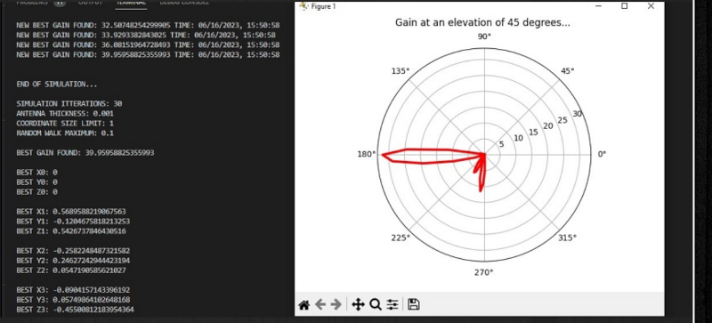
The Python program uses the PyNEC package to provide simulation. The program sets up random antenna lengths and finds the projected gain, attempting to optimize for maximum gain.
The post is long on code and short on details, so you will probably want to read the Python source to see exactly what it is doing. But it could probably serve as a template to do other simulated annealing simulations for other antennas or anything you had a simulation engine to evaluate.
Several techniques allow you to optimize things that are too hard to search exhaustively, and we’ve talked about simulated annealing and genetic algorithms before. However, lately, we’ve been more interested in annealing 3D prints.


Scipy has a lot of general purpose optimisation routines that are a bit more advanced than SA. Basin hopping or Differential Evolution often perform better, specially if you have the CPU cycles to spare.
There is one fun algorithm based on the behaviour of sparrows foraging. Not sure how well it would do antennae.
updated…
http://www.persion.info/projects/antenna_annealing/
I wonder if anyone has thrown AI at the problem
fer shur; here’s a fun one
https://en.wikipedia.org/wiki/Evolved_antenna
that’s just evolutionary searching. pretty much what this article is about. I remember when that antenna they show was in the news way back.
Tbf Wikipedia calls it AI.
“In computer science, evolutionary computation is a family of algorithms for global optimization inspired by biological evolution, and the subfield of artificial intelligence and soft computing studying these algorithms. In technical terms, they are a family of population-based trial and error problem solvers with a metaheuristic or stochastic optimization character.”
Not sure what your criteria for “AI” is then – I doubt a large language model would be a good fit for this. Perhaps a GAN-based approach qualifies? https://ieeexplore.ieee.org/document/9763831
yeah, that looks more like it.
updated…
http://www.persion.info/projects/antenna_annealing/
(I have a phd in combinatorial optimization theory and machine learning). I think these folks are light on math… this is the typical kind of approach a computer scientist or an electrical engineer might try. Folks don’t know anything about Operations Research and that’s the problem. Trying to discretize options and then do a multi dimensional grid search is a worst case outcome. Searching N dimensional haystacks with simulated annealing techniques is no good either.. combinatorics grow even faster than exponentials and the fraction of the search energy that’s doing something useful goes to 0 very, very quickly as the number of dinensions grows. The Curse of Dimensionality, anyone? You’ll never get there. One needs to cover a volume of the N dimensional parameter space with every query not just a point. (You need a basis function a la the hyperplanes used to represent the value function in the Witness algorithm). So you ask how? Here are a few ideas:
1) convexify the optimisation problem using a penalty function and then proceed e.g. via sequential quadratic approximation. If one could some how generate a first order statespace model / forward model of the function of the antenna, that could be very useful. Seeing as it’s no doubt highly non-linear the tricky part is to figure out how to approximate it within a neighborhood.
2) Danzig Wolfe Decomposition and lagrangian relaxation. I used this approach in my dissertation to solve for a resource allocation policy with an oo number of possible energy allocations… and other complexity besides. Too much to get into here. But I explicitly showed why N dimensional grid search is a terrible way to go and how lagrangian relaxation can be used instead. Just need to approximate constraints and break things into subproblems…
3) Duality theory… anyone tried dualizing the optimization problem?
4) Dynamic programming and neuro dynamic programming… anyone tried e.g. value iteration or PBVI or policy iteration?
5) Why don’t deep neural networks get stuck in local minima? Because Prof. Hinton et al figured out how to convexify their loss functions by adding regularization terms that penalize complexity. I think the same idea could apply here. Successive, approximate convexification of a cost function… also brings up column generation and projection methods and barrier methods / benders Decomposition.
6) I’m using multi heuristic A* hybrid path planning at work these days. A* is a form of dynamic programming. Multiple heuristics are used to guide the evolution of the search frontier. I think a similar notion could apply here. However typically dynamic programming applies to sequential decision making problems in time. In this context I think it might be more like sequential decision making problems in space (hmm… I guess it could go either way… I can see how DP could be applied to solve for an antenna shape that would generate a given waveform by starting at the goal waveform and working backwards across time and all the capacitative/inductive effects that express themselves across time as well…). Ie to start from a dipole a radiating in free space with nothing around it and then tracking how the shape of that radiator (and all its other properties…) would need to evolve in order to maintain optimality as one builds up an environment of increasing complexity around it. The DP solution would evidently need to consider all possible allocations of space around this antenna. That can’t be done without first finding subproblems. I think there’s a calculus of variations linkage here, too: find an optimality principle (e.g. an optimal answer is orthogonal to every possible source of error/inefficiency) and then do a bit of sensitivity analysis to see how that approach evolves as the environment becomes more and more complex. It’s a story of successive approximation. But one where the cpu cycles are reserved for modeling the most important characteristics of the problem at each step. Keep the essentials. Suppress the details.
I’m pretty weak at E+M. But I’m quite strong at computation and decent at modeling, optimization and machine learning. It’s a crying shame no one has ever even heard of Opetations Research. That’s what I’m on about… That and that N dimensional grid searches are the quintessentially stupid way to go.
Case and point:
https://ieeexplore.ieee.org/document/5717913?section=abstract
My call sign is KN6KLL
I really wish I could understand a third of what you wrote…
It does sound interesting!
@The Commentor Formerly Known as Ren: then ask a question. I can’t reply to a statement. I think if my advisor or someone smarter than me read what I just wrote they’d properly say “50% of this is B.S. ; you’re stretching”, and I’d respond “okay yes, that’s true, and 50% isn’t…”.
The key themes:
1) decouple the whole problem into subproblems, this is the most powerful problem solving technique of all when it can be applied and it usually applies
2) approximate constraints where necessary
3) use Lagrange multipliers to convert a constrained optimization problem into an unconstrained one
4) avoid discretizing / sampling approaches at all costs, and this means grid search techniques… for N 1 million…
5) look for an orthogonality principle or optimilality principle as a guiding light… and then ride that wave so to speak… forgive my mixing of metaphors
6) any kind of constrained optimization problem such as min c’*x subject to A*x < b where ' represents a transpose, b,c,x are vectors and A is a matrix has an equivalent dualized problem where the min becomes a max and the constraints become variables and vice versa. The problem doesn't have to be linear (but if not then linear algebra breaks down…). Sometimes the original, primal problem is much harder to solve than the dual problem.
7) Constrained optimizations are much harder to solve than unconstrained ones e.g. : "maximize traffic flow while preventing all drivers from driving through red lights and stop signs". With a hard constraint that problem is ~impossible to solve… but if we take the constraint away and instead replace it with a soft constraint / Lagrange multiplier, it becomes doable… people can drive as they please but if they violate the law they may have to pay $$$; that we can enforce. It's hard to force decisions on people that they've yet to make…
8) sometimes there's a relationship between e.g. searching for something, optimizing something, or finding a shortest path between two points in a high dimensional space… so it may not be readily appararent but often by recasting a problem slightly it can fall into a basket of problems that have already been solved in a slightly different context. Which is where people make realizations like "ohh wait, this is just a multi commodity network flow problem" or "this is just a multi dimensional knapsack problem" or "this is just a job shop scheduling problem" or "this could be solved with the Hungarian algorithm (ie have a virtual/metaphorical auction to choose between various contenders)
9) oftentimes you take a known algorithm such as a Fourier transform which is used to transform a signal across time to one across frequency… but there also exists a usage of Fourier transforms that deal with spatial frequency. Ie the model is a mental one and it's basically the case that the notion of time and frequency are up to your interpretation/ whatever you find useful. So I went out on a limb and took models that typically are applied to problems of decision making in discrete stages across time and am asking the question "okay what about a model of decision making in discrete stages across space, ie the shape of an antenna?"
10) feedback control theory teaches us that in order to make a solid plan, we must build the side effects of the plan into the plan itself. So the first step to doing that is to be able to make a forward model to e.g. simulate the state of a system forward through time (where any element in an electrical circuit that contains energy becomes something to keep track of… that element "has state" and figures into the dimension of the overall statespace of the model. The statespace is the minimum amount of information required to describe what the system in question is doing. Imagine you were playing a computer game and you lost power. The statespace of the game is the minimum size set of numbers that would be necessary to recreate where you were in the game before you lost power. That same idea can be applied to a circuit where the capacitors and inductors store energy. E.g. if I recall, I = C dV/dt for a capacitor and V = L dI/dt for an inductor. Each such element figures into the state of the system. Resistors have no state unless we worry about the heat they're dissipating.. which I've rarely seen addressed. Evidently baluns/ununs (which are fairly new to me) get hot and can change behavior in consequence… so those would figure into the statespace of an antenna. Once we have a forward model then we can start figuring out ways to play with it like a puppet / marionette so to speak using the notions of control theory. This system, aka "plant", can also be stuck in as a black box within a neural network or something which does local search techniques to find better configurations. (But local search techniques suffer the same problem that simulated annealing is trying to overcome… searching N dimensional haystacks). Perhaps the biggest advantage of such modeling is in learning what's not convex about the modeling problem at hand and how to potentially convexify it. Convex optimization problems are solved problems; they're easy.
A lot of the phrases just sound like technobabble from Star Trek or something…
“convexify the optimisation problem” to a layman doesn’t sound like it actually means anything.
“Danzig Wolfe Decomposition and lagrangian relaxation” sounds like something Data would say to explain something to do with wormholes.
Is “combinatorial” even a word?
I swear there’s a lot of professions that wouldn’t be needed if they just wrote in English.
You wouldn’t need lawyers if laws weren’t written in legalese.
@Z00111111:
https://web.mit.edu/dimitrib/www/Convexification_Mult.pdf
This is ax example of Danzig Wolfe Decomposition applied to linear programming. When I used it in my dissertation I had sub problems that were full on POMDP problems. (Search for “Tony’s POMDP page” for more on this). The technique is just a fancy name for how to use a divide and conquer strategy quantitatively…
https://youtu.be/RgmQo7A0ZiA
https://en.m.wikipedia.org/wiki/Dantzig%E2%80%93Wolfe_decomposition
Lagrangian Relaxation is harder to explain. I can’t replace 6+ years of graduate school in a few paragraphs. And my whole point for making this original post is that the people working on these types of problems are ignoring the most important tools in the toolbox…
This example again is specific to integer (linear) programming… but Lagrangian Relaxation can be used in non-linear problems as well:
https://youtu.be/TejLWacGvsw
http://www.ens-lyon.fr/DI/wp-content/uploads/2012/01/LagrangianRelax.pdf
You can search for “3 blue 1 brown Lagrange multiplier site:youtube.com” for 5-6 introductory videos there on Lagrange multipliers. They’re well done.
Also:
https://youtu.be/8mjcnxGMwFo
Combinatorial: the word we use to describe the number of arrangements of a thing. Ie the growth of N choose R. ( I don’t know about you but I learned about combinations and permutations in 7th grade…). N choose R = N! / ((N-R)! * R! ) where 3! for example = 3*2*1.
y(N) = N! is a function that grows even faster than y(N) = exp(N)….
https://mathigon.org/world/Combinatorics
Haven’t checked the details of this post (and I guess you’re right about your assessment), but simulated annealing ain’t that bad when done right. Just another good heuristic to tackle highly nonconvex programs.
IIRC Fujitsu made quite a bit of progress in that particular area.
Simulated annealing is an interesting way to approximate an imprecise solution with a lot of input variables. The US FCC used simulated annealing on the task of assigning a complete digital channel (for simulcast) to pair with every full power TV station in the US. Prior to the analysis, it was generally considered that frequency allocation for NTSC analog interferences/spacings were gridlock.
The FCC analysis was based on evaluating the overall solution “temperature” with penalties for the number of TV viewers receiving interference, based on longley rice coverage analysis.
You start with a total random solution. It will be useless. You measure it, store it and do it again. Measure the second. Compare to first and discard the worst one. Do it all again (for all of the channels in the US) and again about 1000 times until it can’t improve.
Take that result as the “seed” for a second run.
The FCC simulated annealing took about a month to run on Sunsoft Fortran 95, Solaris 2.5.1 and a pizza box SPARC.
For each partial solution.
It is pretty amazing what simulated annealing can do.
http://www.persion.info/projects/antenna_annealing/
updated
… that’s all that simulated annealing is? It’s just making the random changes you try less and less over time? I always hear about it in connection with quantum computing and thought it must be something that needs super deep math to even have a clue what it is.
This is a way to do it when you don’t have a quantum annealer, I believe.
http://www.persion.info/projects/antenna_annealing/
updated
I’m reminded of a YouTube video about Newton, and fractals. Finding a local maxima (or minima) depends on where you start, as the article mentions.
If you make a large grid, and track which point the solution moves towards, you get a fractal pattern.
In antenna design, there are physical design limits (space, size, frequency, direction, etc) that should help reduce the overall size of an N dimension matrix. Finding a range of solutions will probably mean comparing solutions, and choosing which design limits are more important.
The Youtube video: https://youtu.be/-RdOwhmqP5s
Thanks.
An animation of results during computing would be great visual understanding.
updated…
with animation…
http://www.persion.info/projects/antenna_annealing/
http://www.persion.info/projects/antenna_annealing/
updated
I did a major update to my software…
http://www.persion.info/projects/antenna_annealing/