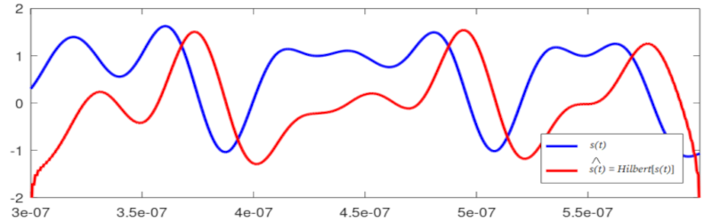
While the Fourier transform gets all the attention, there are other transforms that engineers and mathematicians use to transform signals from one form to another. Sometimes you use a transform to make a signal more amenable to analysis. Other times, you do it because you want to manipulate it, and the transform is easier to change than the original signal. [Electroagenda] explains the Hilbert transform, which is often used to generate single-sideband signals.
The math behind the transformation is pretty hairy. However, if you understand the Fourier transformer, you can multiply the Fourier transform by -i sgn(ω), but that isn’t really going to help you much in a practical sense. If you don’t want to bog down in the math, skip immediately to section two of the post. That’s where it focuses more on the practical effect of the transform. You can think of the transform as a function that produces a 90 degree phase shift with a constant gain. For negative frequencies, the rotation is 90 degrees and for positive frequencies, the shift is negative.
Section 3 shows how mixing a signal with its own Hilbert transform can produce single sideband signals. Typically, a signal is transformed, and the result is multiplied by j (the square root of negative one). When you mix this with the original signal, the negative parts cancel out, while the positive frequencies reinforce each other. If you prefer, you can subtract to get the opposite effect and, thus, the opposite sideband.
There are practical concerns. You must approximate the Hilbert transform, and that will require a filter that has a delay. You’ll need an equalizing delay in the main signal so that the parts that mix together are from the same input time. It also means the phase isn’t as clean as you expect from the theoretical model. If you want to model it all in Matlab, you might find this post enjoyable. If you want a more ham radio take on the same material, check out [K6JCA’s] article on the topic, or watch [ZL2CTM’s] video on the topic below.
If you aren’t ready to swim on the deep end of the signal processing pool, maybe start with some spreadsheets. Once you have a good grip on how IQ can demodulate and modulate, you’ll have an easier time with the Hilbert transform.


I wish HaD did more stuff like this. Much more useful and interesting than seeing how somebody renovated a 50 year old piece of gear that hardly anybody ever used anyway.
Well… Someone must create that content first… :)
I second this, more math explanations, with the technical info and jargon included. I like seeing people stuff raspberry pi’s and arduinos to revive old gear, but I love math even more.
Negative frequency: the rate at which something doesn’t happen.
No, not really. But every time I see that term I’m reminded of that quip from a former coworker.
Ah, just like how negative voltage is how much of an electric shock you *don’t* get from something ;)
Or negative work is doing less than nothing.
“Typically, a signal is transformed, and the result is multiplied by j (the square root of negative one). ” <– Math isn't my forte, but isn't that usually called i?
not when you are talking about voltage (v) and current (i) :)
In electrical engineering, the convention is to use j because i is already reserved for current. My university offered special “for electrical engineers” versions of many math classes, largely because of differing conventions such as this one.
The conventional symbol for current is “I” not “i”. The imaginary unit is usually called “i”. At least that’s how it was when I studied engineering.
It’s “i” because you can confuse I with l which is upper case i with lower case L
Like the iPhone instead of the IPhone.
That is why a proper font like CMU Classical Serif is used for scientific texts. There the problem does not arise at all. Otherwise you start with a clean definition: Let j be the imaginary unit…
Uh, no, because people who write equations *often* want to abuse it and use capital letters for *one* idea of the concept and lowercase for a *different* idea of the concept.
Like, oh, capital I is a *constant* current, but lowercase “i” is a current that varies in time “i(t)”. Or if you’re writing it as a vector, because “I” with the vector-decorator looks weird but “i” with the vector-decorator looks better to you.
There just aren’t enough letters for what people want to do with them. It’s a practical corollary to Guy’s Strong Law of Small Numbers (“there aren’t enough small numbers to meet the many demands made of them” – used to explain why weird small-number patterns show up so often).
Oh no. It’s way, way, way tougher than that.
It’s funny because I can’t really find any source for when engineers started to use “j” instead of “i”. You could say “oh, it’s because of current being I” which, sure, but… well, “I” being used as current isn’t actually that old at all. Ampere’s the one who started using it in France, and it didn’t translate over fully to the rest of the world until the late 19th century.
Maxwell’s entire text on electromagnetism, for instance, doesn’t use “I” for current. When he wrote Ohm’s law, he wrote it as “script E = R*x” (‘script E’ as in the archaic ‘electromotive force’). And of course, he later wrote down his (Maxwell’s) equations in quaternion form, which has three effectively imaginary (as in, their squares are -1) units, labelled… i, j, and k.
And then, of course, Heaviside comes along and writes down equations in a modern vector/tensor basis with i, j, and k being the 3 bases (for x, y, z) – Gibbs also did a lot of the notation, but Heaviside used i, j, k (which we still frequently use). All of this was happening in the late 19th century as well, mind you!
So now you have an interesting point, because if you treat a complex number as a point in a 2D space, you’d typically use “+y” for imaginary… which is “+j”.
So why is it weird to say “well, OK, but avoiding the use of i for current is fine for the 20th century”?
Because guess what symbol Heaviside (whose notation, as noted above, would take over) used for current (which, in his case, was referring to current density)?
Yup. J.
Huh, I might’ve found it. Or I might at least make the case that the “they use j because I is current” is wrong.
One of the first times “complex numbers” comes up to engineers is in Kennelly’s 1893 paper (plus the IEEE discussion) on Impedance. In that paper, Kennelly *never uses* “i” or “j”. He just says “square root of -1” and references “complex numbers.”
He also didn’t use I for current = he used C for current. He used I for *impedance*, which was a very new concept at the time.
There’s an addendum to that paper by Charles Steinmetz which expounds on the use of complex numbers, and in *that* section, he uses “j” for the imaginary unit, while still using C for current and I for impedance.
Of course that’s probably not the first time anyone used “j” for the imaginary unit (…maybe) but it at least shows that when people *were* using it, “I” wasn’t firmly established as meaning “current” yet.
Most of my math education was not electrical engineering, but the rule 40-50 years ago was “Electrical engineers use j instead of i for sqrt(-1)”, though when you did more complicated kinds of numbers you might end up with i,j,k etc.
U.S. pre-WOKE EE here – it is j all-the-way baby!
It is i or j, depending on who you’re talking to. But mixing i and j in a single article is a big no-no. Especially dropping “i” without further explaination and then being smart about “j = sqrt(-1)”.
and here I thought the math was going to be four dimensional using quaternions.
I was always taught that there is no such thing as j=sqrt(-1). Only j^2 = -1. j as a vector, basically.
as trivia, there’s people who use multiple imaginary numbers to make a 4D coordinate space. quaternions. i believe they define i*i=-1, j*j=-1, k*k=-1, but i*j is something more complicated than -1 (they’re *different* square roots of -1).
That’s because they’re vectors, rather than just scalar numbers. The directions of i, j, and k are different.
In the engineering world j is used more often, just call it “i” with a wilted stem…….. [no real reason, just because]
the math articles here always leave me wanting. there are a few related astonishing assertions that can be made quite briefly:
here’s a ridiculous fact: e^(i*pi) = -1. when i first saw it, i was sure it was a joke. there’s a bunch of interesting proofs and narratives for that. i liked the one from Feynmann: https://www.feynmanlectures.caltech.edu/I_22.html
the rough shape of it is he convinces you that e^(i*x) has to be periodic in order to satisfy what we already know about i. and then, he lays it on you: there is the only one periodic function in all of math that has some convenient property like being continually differentiable. sin (and its phase-shifted sibling, cos). so therefore e^(i*x) = cos(x)+i*sin(x). i don’t expect to convince you in a paragraph but just to see this astonishing assertion at the center of it.
Fourier’s story is crazy too. Fourier had a function for the evolution (progressive change as it cools) of temperature along a rod that described what would happen if the initial condition of the rod was the temperature distributed according to an offset sine wave — hotter in the middle, and smoothly cooling to the ends. but he wanted to know how to model the evolution of temperature for more realistic configurations, such as for a rod that was inserted to varying depths into a furnace for some time. instead of (or in addition to) trying to answer that question with physical experimentation, he decided to prove that every signal is equivalent to a combination of sin and cos. not the approach i would have chosen, which is probably why my name won’t be in any math texts!
the Fourier transform itself can be kind of intuitively understood too. a convenient fact from signal processing is that correlation can be established by multiplying 2 signals. suppose they are f(x) and g(x), then if they are identical you get f(x)^2, a strong signal. but if they are not identical, say they are different frequencies, then you will get an interference pattern with a generally smaller magnitude. if they are phase shifted, a different interference pattern. if one is periodic and the other is not, then it can only reduce the magnitude. basically you can use productive interference as a detector. i was thinking about that one day and i imagined, what if you multiplied a sampled signal by sin(x), and sin(2*x) and sin(3*x), or some series like that, so that you correlated it with each member of some frequency series? and to handle out-of-phase situations, maybe you would also do cos(x), cos(2*x), cos(3*x), …?
surprisingly, that is exactly what the Fourier transform is! and that ridiculous e^(i*x)=cos(x)+i*sin(x) above is why multiplying the frequency spectrum by i is a phase shift — it swaps the sin and cos.
Greg, this helped more than most explanations for the Fourier transform that I’ve heard. Thanks!
Hilbert also transforms the bed probing pattern on 3D printers… Supposedly reduces the amount (and time) of travel. But not by my own observations.
Another useful property of the Hilbert transform is that it can be used to estimate the distance between the response of a given network and the response of a nearby causal network since causality has the property of locality. So in estimating the black-box parameters of a passive causal network based upon its reflection coefficients optimizing for causality is a useful search dimension.
Do a search on “Tayloe detector” or “quadrature detector/mixer”. This is how most SDRs generate I&Q baseband audio to feed to the sound card.
The Hilbert Transform is useful for tansmitting and/or receiving Single-Side-Band (SSB) Supressed-Carrier (SC) modulation – amongst other things. More fun here:
1. Chapter 7 Single-Sideband Modulation(SSB) and Frequency Translation
https://user.eng.umd.edu/~tretter/commlab/c6713slides/ch7.pdf
2. Hilbert Transform & Hilbert Spectrum | understanding negative frequencies in the Fourier Transform
https://www.youtube.com/watch?v=dy4OeAYqSqM