It was Stardate 2267. A mysterious life form known as Redjac possessed the computer system of the USS Enterprise. Being well versed in both computer operations and mathematics, [Spock] instructed the computer to compute pi to the last digit. “…the value of pi is a transcendental figure without resolution” he would say. The task of computing pi presents to the computer an infinite process. The computer would have to work on the task forever, eventually forcing the Redjac out.
Calculus relies on infinite processes. And the Arduino is a (single thread) computer. So the idea of  running a calculus function on an Arduino presents a seemingly impossible scenario. In this article, we’re going to explore the idea of using derivative like techniques with a microcontroller. Let us be reminded that the derivative provides an instantaneous rate of change. Getting an instantaneous rate of change when the function is known is easy. However, when you’re working with a microcontroller and varying analog data without a known function, it’s not so easy. Our goal will be to get an average rate of change of the data. And since a microcontroller is many orders of magnitude faster than the rate of change of the incoming data, we can calculate the average rate of change over very small time intervals. Our work will be based on the fact that the average rate of change and instantaneous rate of change are the same over short time intervals.
Houston, We Have a Problem
In the second article of this series, there was a section at the end called “Extra Credit” that presented a problem and challenged the reader to solve it. Today, we are going to solve that problem. It goes something like this:
We have a machine that adds a liquid into a closed container. The machine calculates the amount of liquid being added by measuring the pressure change inside the container. Boyle’s Law, a very old basic gas law, says that the pressure in a closed container is inversely proportional to the container’s volume. If we make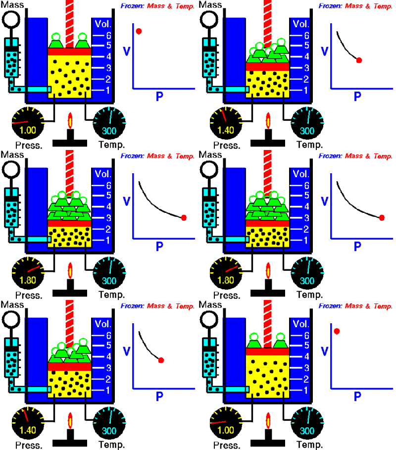 the container smaller, the pressure inside it will go up. Because liquid cannot be compressed, introducing liquid into the container effectively makes the container smaller, resulting in an increase in pressure. We then correlate the increase in pressure to the volume of liquid added to get a calibration curve.
The problem is sometimes the liquid runs out, and gas gets injected into the container instead. When this happens, the machine becomes non-functional. We need a way to tell when gas gets into the container so we can stop the machine and alert the user that there is no more liquid.
One way of doing this is to use the fact that the pressure in the container will increase at a much greater rate when gas is being added as opposed to liquid. If we can measure the rate of change of the pressure in the container during an add, we can differentiate between a gas and a liquid.
Quick Review of the Derivative
Before we get started, let’s do a quick review on how the derivative works. We go into great detail about the derivative here, but we’ll summarize the idea in the following paragraphs.
An average rate of change is a change in position over a change in time. Speed is an example of a rate of change. For example, a car traveling at 50 miles per hour is changing its position at 50 mile intervals every hour. The derivative gives us an instantaneous rate of change. It does this by getting the average rate of change while making the time intervals between measurements increasingly smaller.
Let us imagine a car is at mile marker one at time zero. An hour later, it is at mile marker 51. We deduce that the average speed of the car was 50 miles per hour. What is the speed at mile marker one? How do we calculate that? [Issac Newton] would advise us to start getting the average speeds in smaller time intervals. We just calculated the average speed between mile marker 1 and 51. Let’s calculate the average speed between mile marker’s 1 and 2. And then mile marker’s 1 and 1.1. And then 1 and 1.01, then, 1.001…etc. As we make the interval between measurements smaller and smaller, we begin to converge on the instantaneous speed at mile marker one. This is the basic principle behind the derivative.
Average Rate of Change
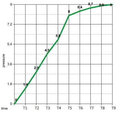
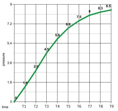
We can use a similar process with our pressure measurements to distinguish between a gas and a liquid. The rate of change units for this process is PSI per second. We need to calculate this rate as the liquid is being added. If it gets too high, we know gas has entered the container. First, we need some data to work with. Let us make two controls. One will give us the pressure data for a normal liquid add, as seen in the graph above and to the left. The other is the pressure data when the liquid runs out, shown in the graph on the right. Visually, it’s easy to see when gas gets in the system. We see a surge between time’s T4 and T5. If we calculate the average rate of change between 1 second time intervals, we see that all but one of them are less that 2 psi/sec. Between time’s 4 and 5 on the gas graph, the average rate of change is 2.2 psi/sec. The next highest change is 1.6 psi/sec between times T2 and T3.
So now we know what we need to do. Monitor the rates of change and error out when it gets above 2 psi/sec.
Our psuedo code would look something like:
x = pressure;
delay(1000);
y = pressure;
rateOfChange = (y - x);
if (rateOfChange > 2)
    digitalWrite(13, HIGH);  //stop machine and sound alarm
Instantaneous Rate of Change
It appears that looking at the average rate of change over a 1 second time interval is all we need to solve our problem. If we wanted to get an instantaneous rate of change at a specific time, we need to make that 1 second time interval smaller. Let us remember that our microcontroller is much faster than the changing pressure data. This gives us the ability to calculate an average rate of change over very small time intervals. If we make them small enough, the average rate of change and instantaneous rate of change are essentially the same.
Therefore, all we need to do to get our derivative is make the delay smaller, say 50ms. You can’t make it too small, or your rate of change will be zero. The delay value would need to be tailored to the specific machine by some old fashioned trial and error.
Taking the Limit in a Microcontroller?
One thing we have not touched on is the idea of the limit within a microcontroller. Mainly, because we don’t need it. Going back to our car example, if we can calculate the average speed of the car between mile marker one and mile marker 0.0001, why do we need to go though a limiting process? We already have our instantaneous rate of change with the single calculation.
One can argue that the idea behind the derivative is to converge on a single number while going though a limiting process. Is it possible to do this with incoming data of no known function? Let’s try, shall we? We can take advantage of the large gap between the incoming data’s rate of change and the processor’s speed to formulate a plan.
Let’s revisit our original problem and set up an array. We’ll fill the array with pressure data every 10ms. We wait 2 seconds and obtain 200 data points. Our goal is to get the instantaneous rate of change of the middle data point by taking a limit and converging on a single number.
We start by calculating the average rate of change between data points 100 and 200. We save the value to a variable. We then get the rate of change between points 100 and 150. We then compare our result to our previous rate by taking the difference. We continue this process of getting the rate of change between increasingly smaller amounts of time (from the 100th data point) and comparing them by taking the difference. When the difference is a very small number, we know we have converged on a single value.
We then repeat the process in the opposite direction. We calculate the average rate of change between data points 0 and 100. Then 25 and 100. Then 50 and 100 and so on. We continue the process just as before until we converge on a single number.
If our idea works, we’ll come up with two values that would look something like 1.3999 and 1.4001 We say our instantaneous rate of change at T1 is 1.4 psi per second. Then we just keep repeating this process.
Now it’s your turn. Think you have the chops to code this limiting process?






That code sample should be:
x = pressure;
delay(1000);
y = pressure;
That code snippet should be:
x = pressure;
delay(1000);
y = pressure;
Right you are, fixed. Thanks!
“We continue this process of getting the rate of change between increasingly smaller amounts of time”
This makes the process more and more sensitive to noise.
“Let us imagine a car is at mile marker one at time zero. An hour later, it is at mile marker 50. We deduce that the average speed of the car was 50 miles per hour. ”
I believe you mean mile marker *zero* at time zero. Otherwise the average speed is 49 miles per hour.
Fixed. Thanks!
you’re not asking us to do your homework are you?
My intention was to code the limit idea but I failed miserably. It would be neat if someone could do it, though. I don’t think anyone ever has. I’m not sure how useful it would be. But it would be pretty cool to “take the limit” of an analog pin. I’m not sure if it’s even possible.
As the delta t gets very small you will run into the electron statistics until you get wild variation – 1 electron, 3 electrons, no electrons, 7 electrons – in your intervals, and it will fall apart. Limits need continuous functions, you can approximate but have to know the math of the noise and quantum effects if you use electric current in an example.
I’ve done this before to create a PID controller using an Arduino. It really isn’t as hard as everyone’s making it out to be. When computing integrals or derivatives of live data you don’t even WANT to use limits. The actual calculation is just simple arithmetic. If your signal is very noisy you first take averages of data points or whatever to get at your trusted values. You will have an array or queue of these running values. Then you determine what you want your time interval to be. A larger interval will also reject more noise. Calculate the derivative by taking your “current” value, subtract the historic value, and divide by your time interval. Choose an interval that’s a power of 2 so you can do division quickly by bit-shifting alone. This is how it’s done in the real world.
Think about it this way – no sensor system will produce a continuous function by sampling data n times per second, no matter how large n is. We know from calculus you can only take a derivative of a continuous function. So you should see it is impossible to “take the limit of an analog pin”.
That sounds a lot like an FIR filter.
Yeah…when I was thinking it through I didn’t really see the need for a limiting process. But I thought I should at least mention it and come up with a rough idea on how to do it.
LOL! Cynic…
The last digit of Pi would be zero in base Pi.
Except when you try to construct a number system in base Pi it quickly falls apart when you realize many numbers have infinitely different representations, or to put it another way, pretty much any number you write down will not be unique. So in practice a number system in base Pi is not possible.
The figure shows Pi! or Pi Factorial. Let me do a little Gamma function calculation in my head …. yeah. Pi! is about 7.188 If you read this far you are a total Trek nerd and I bet you argue about Kirk versus Picard – as if it isn’t obvious.
There’s something on the wing, some thing!
If we can measure the rate of change of the pressure in the container during an add, we can differentiate between a gas and a liquid.
differentiate
Was that a pun right there? ;)
only if you’d said ‘differentialate’, but I think that’s actually a portmanteau. Sometimes a portmaneteau can be classed as a pun. Not sure if this qualifies
I didn’t get a chance to read the entire thing top to bottom, my only question is how is a single threat microcontroller suppose to keep track of miles travel if it is also doing other tasks? Would a odometer not be a job for a arduino that controllers many other things inside my car?
any interrupt is a threat :)
The rate of change is (y-x)/1000. (y-x) is just the change. Be careful!
wasn’t it about that if the change was to big, there would be gas inside the container/machine ?
Haven’t you got the best answer you’re going to get, by using a weighted average of as many samples as you can take within a reasonable, defined calibration period. Might not be *the limit*, but surely it’ll be good enough?
“π!” is an oxymoron because the exclamation mark has a math function (factorial) that can only operate on integers.
https://en.wikipedia.org/wiki/Gamma_function
>In mathematics, the gamma function (represented by the capital Greek letter Γ) is an extension of the factorial function, with its argument shifted down by 1, to real and complex numbers.
This is why I hated physics in high school, and loved it in college. Or even geometry! 2πr, πr², F=MA but EK = ½mv²? Without calculus, those are just formula that you memorize. With calculus, they are the beautiful ways that all of those concepts are interconnected.
Frankly, I wish I could have taken calculus earlier in school. A great 7th grade teacher ran our class through algebra and geometry (and told us that is what the math was, didn’t hide it behind anything) at the end of each 6-weeks if we finished the assigned stuff ahead of time. We touched on calculus by doing string art (like http://mathforum.org/mathimages/imgUpload/thumb/X%5E2_string.gif/400px-X%5E2_string.gif) and explaining that we were seeing the slope of the line at the point where it was tangent. “Slope” is an easy word here, we’re on mountains, and tangent she just called a point. Had we been able to get more of that information in my head before taking geometry and then trig, I think those would have been interesting instead of just “memorize, test, forget”.
Though, you do end up needing trig stuff for more interesting calculus, and that requires a foundation of geometry. So I know why it’s taught in that order, I just wish it wasn’t.
This is why I hated Calculus in college and loved it in grad school. The different rules of Calculus are just things you memorize. The divergence theorem, fundamental theorem of calculus, and Green’s Theorem seem like different concepts. But with Stokes’ Theorem you see how they are beautifully interconnected. Frankly, I think they should just teach differential forms earlier in school. ;)
Considering the TI calculators run Z80 and do advanced maths, an AVR can do the same
except that the run faster? don’t think it’s just running the z80 at 4MHz or so!
As with the previous article, lots of comments but no one doing the homework. Here’s a quick stab at it, please tell me where I’ve gone wrong (obviously this is only the upper value).
int arrayPos = 200; // array position int decAmount = 100; // amount to decrement array position by float change = 0; float rate = 10000; // rate, initialise large to begin while loop float prevrate = 0; // store previous rate for comparison float limit = 0.1; // set how finer limit we want to work too while ( (prevrate - rate) > limit ) { prevrate = rate; // store rate for comparison next time around change = presArray[arrayPosition] - presArray[arrayPos - decAmount]; rate = change / (arrayPos - decAmount); // should get everything in same per unit time decAmount /= 2; // reduce decrement amount by half arrayPos -= decAmount; // reduce array position for next loop }Thanks for this! Good stuff!
It would be great if hackaday staff could mod the comments for code if its possible. I had indents that have gone :(
Try putting your code in pre tags
Nice, thanks for the fix. Didn’t know they worked on here. Now I feel foolish :s
The general idea is to fit a polynomial to the data in the area of interest and then calculate an exact derivative from that polynomial. My understanding is that most all of numerical analysis is based on fitting a polynomial as best as possible and then doing the math on that.
There is tradeoff in diminishing the interval between getting a more accurate picture of the slope at the exact point where the derivative is wanted and diminishing numerical precision from truncation in the calculations. I think I would fit a second order polynomial centered on the point of interest with at least 100 A/D counts difference above and below.
Then calculate the derivative of this and evaluate it at the point. Note that the derivative can be formed in software directly from the poly.
f(x) = a*x^2 + b*x + c
f'(x) = 2*a*x + b
Indeed, numerical analysis is the way to go. It has to be taken into account also though, that an interpolating polynomial is not automatically monotonicity preserving on intervals with local extrema. This can cause problems because the interpolant will have differing monotonicity from the recorded data around nodes with local extrema which will cause the computed derivative to have the wrong sign in these regions. This asks for piecewise polynomial interpolation with local slope limiting to get local monotonicity preservation, for example with cubic hermite polynomials; setting the slope values to zero for data nodes representing extrema will do the trick.
Construction and evaluation of this kind of polynomial should both be possible in linear time.
If I was to actually implement this I would do this.
In = (A_D read)<>2 // low pass filters the DIff for noise
Xold = In
DiffOut = Diffav>>4
This implements a differentiator followed by a lowpass filter.
The lowpass filter output is updated by the Difference /4
never mind formatting destroyed the comment.