In the early 20th century, Guinness breweries in Dublin had a policy of hiring the best graduates from Oxford and Cambridge to improve their industrial processes. At the time, it was considered a trade secret that they were using statistical methods to improve their process and product.
One problem they were having was that the z-test (a commonly used test at the time) required large sample sizes, and sufficient data was often unavailable. By studying the properties of small sample sizes, William Sealy Gosset developed a statistical test that required fewer samples to produce a reasonable result. As the story goes though, chemists at Guinness were forbidden from publishing their findings.
So he did what many of us would do: realizing the finding was important to disseminate, he adopted a pseudonym (‘Student’) and published it. Even though we now know who developed the test, it’s still called “Student’s t-test” and it remains widely used across scientific disciplines.
It’s a cute little story of math, anonymity, and beer… but what can we do with it? As it turns out, it’s something we could probably all be using more often, given the number of Internet-connected sensors we’ve been playing with. Today our goal is to cover hypothesis testing and the basic z-test, as these are fundamental to understanding how the t-test works. We’ll return to the t-test soon — with real data.
I recently purchased two of the popular DHT11 temperature-humidity sensors. The datasheet (PDF warning) says that they are accurate to +/- 2 degrees C and 5% relative humidity within a certain range. That’s fine and good, but does that mean the two specific sensors I’ve purchased will produce significantly different results under the same conditions? Different enough to affect how I would use them? Before we discuss how to quantify that, we’ll have to go over some basic statistical theory. If you’ve never studied statistics before, it can be less than intuitive, so we’ll go over a more basic test before getting into the details of Student’s t-test.
It’s worth starting by mentioning that there are two major schools of statistics – Bayesian and Frequentist (and there’s a bit of a holy war between them). A detailed discussion of each does not belong here, although if you want to know more this article provides a reasonable summary. Or if you prefer a comic, this one should do. What’s important to remember is that while our test will rely upon the frequentist interpretation of statistics, there are other correct ways of approaching the problem.
For our example, imagine for a moment you are working quality control in a factory that makes 100 Ω resistors. The machinery is never perfect, so while the average value of the resistors produced is 100 Ω, individual resistors have slightly different values. A measure of the spread of the individual values around the 100 Ω average is the standard deviation (σ). If your machine is working correctly, you would probably also notice that there are fewer resistors with very high deviations from 100 Ω, and more resistors closer to 100 Ω. If you were to graph the number of resistors produced of each value, you would probably get something that looks like this:
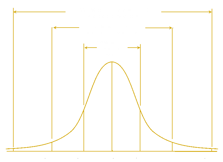
This is a bell curve, also called a normal or Gaussian distribution, which you have probably seen before. If you were very astute, you might also notice that 95% of your resistor values are within two standard deviations of our average value of 100 Ω. If you were particularly determined, you could even make a table for later reference defining what proportion of resistors would be produced within different standard deviations from the mean. Luckily for us, such tables already exist for normally distributed data, and are used for the most basic of hypothesis tests: the z-test.
Let’s say you then bought a machine that produces 100 Ω resistors — you quit your job in QC and have your own factory now. The vendor seemed a bit shady though, and you suspect the machine might actually be defective and produce resistors centered on a slightly different value. To work this out, there are four steps: develop a set of hypotheses, sample data, check if the sampled data meets the assumptions of your test, then run the test.
Developing Hypotheses
There are only two possibilities in our case: the machine either produces resistors that are significantly different from 100 Ω, or it doesn’t. More formally you have the following hypotheses:
H0: The machine does not produce resistors that are significantly different from 100 Ω
HA: The machine produces resistors that are significantly different from 100 Ω
H0 is called our null hypothesis. In classical statistics, it’s the baseline, or the hypothesis to which you’d like to give the benefit of the doubt. Here, it’s the hypothesis that we don’t find a difference between the two machines. We don’t want to go complaining to the manufacturer unless we have clear evidence that the machine isn’t making good resistors.
What we will do is use a z-score table to determine the probability that some sample we take is consistent with H0. If the probability is too low, we will decide that H0 is unlikely to be true. Since the only alternative hypothesis is HA, we then decide to accept HA as true.
As part of developing your hypotheses, you will need to decide how certain you want to be of your result. A common value is 95% certainty (also written as α=0.05), but higher or lower certainty is perfectly valid. Since in our situation we’re accusing someone of selling us shoddy goods, let’s try to be quite certain first and be 99% sure (α=0.01). You should decide this in advance and stick to it – although no one can really check that you did. You’d only be lying to yourself though, it’s up to your readers to decide whether your result is strong enough to be convincing.
Sampling and Checking Assumptions
Next you take a random sample of your data. Lets say you measure the resistance of 400 resistors with your very accurate multimeter, and find that the average resistance is 100.5 Ω, with a standard deviation of 1 Ω.
The first step is to check if your data is approximately shaped like a bell curve. Unless you’ve purchased a statistical software package, the easiest way I’ve found to do this is using the scipy stats package in Python:
import scipy.stats as stats

list_containing_data=[]

result = stats.normaltest(list_containing_data)

print result
As a very general rule, if the result (output as the ‘pvalue’) is more than 0.05, you’re fine to continue. Otherwise, you’ll need to either choose a test that doesn’t assume a particular data distribution or apply a transformation to your data — we’ll discuss both in a few days. As a side note, testing for normality is sometimes ignored when required, and the results published anyway. So if your friend forgot to do this, be nice and help them out – no one wants this pointed out for the first time publicly (e.g. a thesis defense or after a paper is published).
Performing the Test
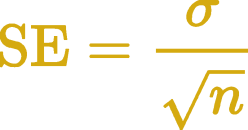
Now that the hard part is over, we can do the rest by hand. To run the test, we determine how many standard errors away from 100 Ω the our sample average is. The standard error is the standard deviation divided by the square root of the sample size. This is why bigger sample sizes let you be more certain of your results – everything else being equal, as sample size increases your standard error decreases. In our case the standard error is 0.05 Ω.
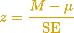
Next we calculate the test statistic, z. This is the difference between the sample mean of 100.5 Ω and the value we’re testing against of 100 Ω, divided by the standard error. That gives us a z value of 10, which is rather large as z-statistic tables typically only go up to 3.49. This means the probability (p) of obtaining our observed sample is less than 0.001 (or less than 0.1% if you prefer) given that the null hypothesis is true. We would normally report this as p < 0.001, as no one really cares what the precise value of p is when it’s that small.
What Does it Mean?
Since our calculated p is lower than our threshold α value of 0.01 we reject the null hypothesis that the average value of resistors produced by the machine is 100 Ω… there’s definitely an offset, but do we call our vendor?
In real life, statistical significance is only part of the equation. The rest is effect size. So yes, our machine is significantly off specification… but with a standard deviation of 1 Ω, it wasn’t supposed to be good enough to produce 1% tolerance resistors anyway. Even though we’ve shown that the true average value is higher than 100 Ω, it’s still close enough that the resistors could easily be sold as 5% tolerance. So while the result is significant, the (fictional) economic reality is that it probably isn’t relevant.
This is all well and good for our fictional example, but in real life data tends to be expensive and time-consuming to collect. As hackers, we often have very limited resources. This is an important limitation to the z-test we’ve covered today, which requires a relatively large sample size. While Internet-connected sensors and data logging are inexpensive these days, a test that puts more knowledge within the reach of our budget would be great.
We’ll return in a short while to cover exactly how you can achieve that using a t-test, with examples in Python using a real data set from IoT sensors.


“In the early 20th century, Guinness breweries in Dublin had a policy of hiring the best graduates from Oxford and Cambridge to improve their industrial processes. At the time, it was considered a trade secret that they were using statistical methods to improve their process and product.”
Where’s Deming when you need him? :-D
I take issue with the explanation given above. While technically correct, it gives the reader no inkling of why the calculations are done or what the meanings are.
Basically, if you want to test something (a hypothesis), take a lot of samples, run this named subroutine thingy, divide this by that, and compare it to some numbers given in the text. If you’re p is less than 0.05, you’re good.
This causes all sorts of problems in the literature, because it leads to scientists doing the calculations by rote. They go through all the steps, get an output, and publish, but have no real understanding of what’s happening or why they are doing it.
If you don’t have an understanding of where the numbers come from, it’s impossible to tell when you have made a mistake.
Let’s turn it around and explain it a different way.
Suppose flipping a coin ten times comes up heads eight times. Is the coin fair?
In reality we can never know whether the coin is actually fair, because even a fair coin will come up heads 8 times (in ten trials) occasionally. What we need to do is compare the results (8 heads in 10 trials) with what an actual fair coin does and see how likely this result is.
So we get a fair coin and flip it 10 times and note the number of heads. We do this again, and again, and again… and after a million trials (using a computer) we tally the results and compare with our suspect coin.
Our computerized tally shows that a fair coin comes up 8 heads or more about 5.47% of the total trials.
So now we need a rule that tells us how much suspicion we need before we reject the coin as biased. In the example above, we have a 94.53% chance that the coin is biased, and 5.47% that it is fair: do we accept this as significant?
This is the infamous “p” value, and there’s a gentleman’s agreement that 5% is considered significant (p < 0.05, or a 5% chance that the results are due to randomness), meaning that you can publish results. That's a 1-in-20 chance of publishing results that are due to chance; and by extension, about 1 in 20 statistical studies in the literature are reporting chance results.
There is no fundamental reason to use the 5% value, and some fields use different values. For example, a drug trial – where patients could die – might use p < 0.01 for extra certainty. Physicists use a 1-in-3.5 million value when reporting results. (Because the equipment is expensive, and experiments are difficult to reproduce. Physicists take pains to get it right the first time.)
Regarding the article, the "do this by rote" manner of explanation is OK and technically correct, but the "this is what's actually happening" explanation leads to better understanding, and will reduce the risk of researchers making errors of logic.
With the "simulate a million trials" explanation the researcher could in theory do the calculation without the library package. With the explanation as posted, if the researcher had no access to the statistical function, they they would have no way to gauge their results.
I take issue with this because there's a bunch of problems in the scientific literature right now, and this is one of them. Many, many researchers have no commonsense understanding of the statistical tests they are using, and simply apply them by rote.
We could mitigate this problem on the hackaday journal somewhat by being more clear in our explanations and note why to do things a certain way.
Those are all good points, but this was supposed to be a short introduction, and I think it achieved that end well.
When I worked (i.e. before I retired), our products were made for the FAA. On one program I worked, the FAA created a 4th or 5th generation of a technical equipment spec and corresponding testing (in this case, an ILS system) that allocated errors to subsystem elements that were never fully decomposed or attributed to their source. This resulted in many “failed” tests, delivery delays, nearly a contract cancellation, and a lot of ill will. The authors of the original FAA specs and tests were long deceased and NO ONE fully knew what the true purpose for all the tests were anymore. Of course, this all hid behind a facade of “statistics” that made our equipment (and hence my work on it) “bad”. There was no “arguing” the fact, as the newbie technical experts with no prior ILS knowledge “tweaked” prior test procedures to address “better technology” and the ability to achieve “higher performance standards” without knowing what that REALLY entailed. It was a nightmare best forgotten (but my former colleagues still struggle under that shroud).
I’m generally with you — taking a 5% p-val and calling it a success is a copout. Don’t get me started on implicit multiple hypotheses and cherry-picking.
That said, Sean _did_ actually justify picking a 1% cutoff in this case, went into the rationale behind framing the null and alternative, and even covered effect size vs. significance. And all of this in a lay-persony way, and a short(ish) writeup. I thought that was pretty darn impressive.
You can legitimately cherry-pick from multiple hypotheses if apply the corresponding Bonferroni correction. But I know what you mean. ;)
Bonferroni is just dividing the p-value by N, where N is the number of hypotheses. It’s extremely conservative when hypotheses are correlated — and thus not a very powerful/practical test. The “overall-F” type tests are much more powerful, but the alternative hypothesis (“at least one of the multiple null hypotheses is false”) is often uninteresting.
There are tons of interesting multiple hypothesis tests between these two extremes. I’m a really big fan of the “false discovery rate” idea — no more than a specified percent of the rejected null hypotheses will turn out to be actually null. I did some work on these tests and applications in econometrics, and now you have to call me “Dr. Elliot”.
Just sayin. :) I loves me some multiple hypothis testing.
Scientists are having a hard time reproducing studies, indicating that it is often the chance results that are being chosen for publishing.
“That’s a 1-in-20 chance of publishing results that are due to chance; and by extension, about 1 in 20 statistical studies in the literature are reporting chance results.”
That is the terrible assumption that leads to p-hacking and the generally low quality of a lot of empirical publications. There is a 1-in-20 chance of any given p<0.05 test coming up with a false positive in the presence of no relationship between the quantities. Say I select 20 spurious relationships ("the reduction in naval piracy is related to global warming", etc) and run the t-test on those relationships, I would expect to get approximately one (false) result showing a statistically significant relationship, which I would then publish. I repeat this process until I get bored, testing loads of crap hypotheses and publishing the lucky 5%… so 100% of the results that I publish will be false positives.
This sort of thing is why there is a big push (see also: Ben Goldacre) for medical studies to publish the hypotheses that they will test before gathering data. Where any study claims a statistical relationship post-hoc, i.e. by inspection of the data, there is a very high probability that that relationship is spurious.
Some lovely examples: http://www.tylervigen.com/spurious-correlations
FWIW I think in much of particle physics, the standard is a 5-sigma result before publishing. They also have a habit of testing hypotheses arising from theory rather than (I presume…) just combing through their data.
Not arguing with the point that the 0.05 bar is to low but.
“That’s a 1-in-20 chance of publishing results that are due to chance; and by extension, about 1 in 20 statistical studies in the literature are reporting chance results.”
Your statement is only true if all the p values in each study are exactly 0.05. This is not the case and many are significantly higher.
It would be awesome if only 5% of published papers were “wrong” because they rejected true null hypotheses.
Here’s an old scam: send out a newsletter to 2000 people — 1000 saying Apple stock will go up today, and 1000 saying it will go down. Send out newsletters to the recipients who received the correct prediction with another 50/50 prediction. Repeat. In the end, some people will be like “wow, he made 10 correct predictions in a row!” and buy your stock advice.
Mulitple potential (scientific) effects are the stock tips. Publishing the one that made it through is survivorship bias. That journals like to publish significant results is publication bias. That the rate, in some fields, is as high as 30% or more is proof that these effects matter.
There is no statistical solution to this, sadly. Enforcing higher confidence just makes the scientists run more tests before finding a “significant” one, or in fields where data is scarce will kill off actual results unnecessarily.
Replication and a culture of verification can help. Openness about the procedures and the research paths not chosen can also shed additional light on the matter. How many non-starters were considered before the one significant effect was discovered? Etc. Encouraging statistical literacy among scientists can’t hurt, and it will eventually trickle down to the journals. (I think it’s actually happening, over the last decade or so.)
This is a real problem in science right now, and the answers are not easy. But publication bias is waaaay more of a deal than just picking 1% vs 5% p-vals. Like orders of magnitude more.
I agree with you more or less across the board. Alpha values (“significance”) are especially problematic in science right now, and I’m happy to see this type of discourse happening here. Overall I think p/alpha values rely too much on everyone being perfectly honest (including to themselves). Maybe we can do better?
If it were up to me we’d drop the concept of statistical significance entirely — report your p-value and effect size, then let the reader decide if it’s good enough for them. Also some type of requirement for the data to be stored somewhere accessible — not so much for honesty as meta-analysis.
I have to admit though that my interest in statistics started with learning a couple of tests by rote. Those simple tests are often useful to me just the way they are. If the only tool you have is a hammer, that’s OK if all you need to do is affix a nail, I guess. If you accumulate tools like I do, you’ll soon have more anyway!
To be honest, I had a hard time finding a starting point to write about statistics, so I decided to start with sharing a simple tool. I hope that with time, I’ll be able to touch on the concerns you’ve raised because they are valid, important, and interesting.
Nice overview. I always assumed that Student was a person’s actual name! It was good to point out the normality requirement as a lot of statistical analysis only works effectively when the variations are random or close to random. Systemic failures generally behave differently.
Z-score or t-test is fine for a quick check. It’s nice if experiment is repeatable, you have relatively large sample, and the sample size was set before experiment, and you decided about all tests that you want to do before starting analysis. If you don’t have this kind of setup, then testing for normality becomes just one of the smaller problems that you run into using to null hypothesis significance testing (NHST).
What if your sample size is one and there is no way of repeating the experiment, but you have some prior knowledge?
Here is a very nice paper about bayesian replacement of t-test: http://www.indiana.edu/~kruschke/publications.html (Bayesian estimation supersedes t-test).
This comment is no place for explanation why bayesian estimation makes so much more sense for me, but in short: for the price of a bit more difficult model setup, longer computation time and more memory used I get the benefit of knowing both magnitude and uncertainty of my estimates and I have the possibility to perform all kinds of comparisons at once, also with magnitude and uncertainty of differences between groups.
For anyone interested in bayesian approach, I highly recommend books and blogs of John Kruschke and Andrew Gelman.
I wish I had known about all of this earlier and not waste my time on choosing the correct NHST test, p-values, bootstraping, and confidence intervals.
Bayesian vs Classical/Frequentist: add another holy-war topic to the Hackaday list! :)
The issue with Bayesian hypothesis testing is that if different people have different priors, they’ll reach different conclusions about the test results — assuming they can calculate them. The issue with classical hypothesis testing is that it doesn’t take the investigator’s prior knowledge into account. One coin, two sides.
As for your hypothetical question: if your sample size is one? You really, badly, need more data. No prior belief you can hold will convince me. With one data point, you can estimate a mean. But what’s the std dev of that estimate? Hint: you’re dividing by N-1.
Anyway, if you’re getting seriously into stats, you’re going to want to be familiar with both perspectives. At the end of the day, the point of a hypothesis test is to convince an audience that something is significant, or to make a decision that minimizes some measure of loss. Which paradigm is appropriate is not always up to you.
Totally second the recommendation of Andrew Gelman. (John Kruschke is new to me.)
of course classical NHST has priors. it just covers them up and pretends they’re not there.
you’ve misunderstood (or miscommunicated) the meaning of a p-value. don’t feel bad, it’s distressingly common.
https://en.wikipedia.org/wiki/Misunderstandings_of_p-values
an introduction to using Stan for this sort of problem would be valuable; it’s simpler than all the frequentist rituals, and you end up with answers that everyday folk can actually use.
Thanks for catching that, I see the offending sentence. It’s one of those things that’s a basic error but easy to write by accident. I’ll make a correction shortly.
For posterity, the article originally stated “This means the probability (p) that our null hypothesis is correct is less than 0.001 (or less than 0.1% if you prefer).”
The p value does not indicate the probability that the null hypothesis is true/correct. The p value measures the probability of observing the effect that we did, given that the null hypothesis is true.
One important effect of the above is that if you ever get a very high p-value (say, 0.96) then you have not proven the null hypothesis — you have only failed to reject it.
“(PDF warning)”
I appreciate the “PDF” part but could really do without the “warning”…
Glancing at the data sheet for the DHT11, this looks like a pretty crappy part. Accuracy +/- 2C isn’t really very good. I know it’s apples and oranges, but the old LM35 temperature sensor was good for +/- 0.5C
Where in the datasheet does it specify the Tmax and Tmin that the part operates over? Same for the Humidity. What range of humidities is it good for? The bit format says that 8-bits specify the temperature’s integer part, and and additional 8-bits for the fractional part. I seriously doubt this device is good to 1/256 of a degree precision.
As I recall the operating range is 0-50 degrees Celsius and 20-80% relative humidity. The datasheet from adafruit for it said so but I couldn’t access it recently for some reason.
I suspect it is so inaccurate because it uses 2 thermistors to measure temperature internally, and then the temperature measurement is used to calculate the RH. Sometimes they are good enough though, and the price is excellent (just under USD 2$ where I live)
I chose them for this project because they seemed likely to vary a lot between sensors so I’d have something to analyze. If you’re looking for a better sensor then there are a lot out there, even on a low budget. For example, the quite similar DHT-22 uses a more accurate temperature sensor, good to +/- 0.5 degrees C and +/- 1% RH. It’s also good from -40 to 80 degrees C and 0-100% RH.
There are probably many other good choices but those were the two I had on hand. I’ve also used PT100 temperature-dependent resistors to good effect when high accuracy and range was more important than convenience and price.