
Circuit VR is where we talk about a circuit and examine how it works in simulation with LT Spice. This time we are looking at a common low-frequency oscillator known as the Wien bridge oscillator.
What makes an oscillator oscillate? A circuit with amplification that gets the same amount of the output signal fed back into its input, in phase, will oscillate. This is the Barkhausen criterion. Here, we’re going to look into what makes an oscillator work in simulation, and gain some insight into what happens when there’s too much feedback and too little.
In particular, we’ll look at the Wien bridge oscillator, a very simple design that originated as a way to measure impedance back in 1891. Modern versions add some additional features, but let’s start with the most simple implementation and work our way up.
Basics
If you think about the Barkhausen criteria, it is obvious we are going to have an amplifier in the middle of our oscillator. That makes sense. Without amplification, the signal would eventually die away from loss. You can think of an oscillator as an amplifier that keeps re-amplifying its output at a certain frequency — sort of an electronic perpetual motion machine. Of course, the extra energy comes from the amplifier, so no physical laws are being broken, and as long as there’s external power it will run.
Our circuit will consist of an amplifier and a filter circuit. In contrast to some other oscillators which use inverting amplifiers, the Wien bridge uses a non-inverting amplifier. Inverting a signal is equivalent to adding a 180-degree phase shift, which means that the filter network needs to come up with an additional 180 degrees to match the input and output phases. With the Wien bridge, the amplifier is non-inverting, so we need a filter circuit with zero phase shift. Let’s see how that plays out.
Networking
 Consider this schematic (you can download
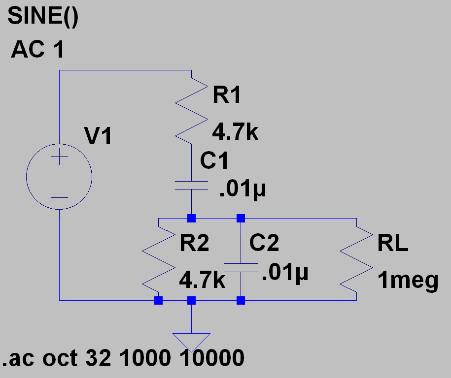
 wien-network.asc from GitHub). With Spice, notice that V1 is just a placeholder that tells the analysis code where to sweep the frequency. RL, of course, is just a load resistor and doesn’t affect the operation of the circuit.
R1 and C1 form a high pass filter. At low frequencies, C1 will tend to block signals. R2 and C2 form a low pass filter. At high frequencies, C2 will approach a short to ground. That means the combined network acts as a bandpass filter. The maximum signal will occur at the frequency when the reactance of C1 is the same as the value of R1. Since I used all the same values, that will be the same frequency where C2‘s reactance is the same as R2‘s value.
If the resistance and the reactance are equal at some frequency, it makes sense that the phase shift will be zero at the same frequency. You can pretty quickly calculate: 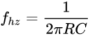
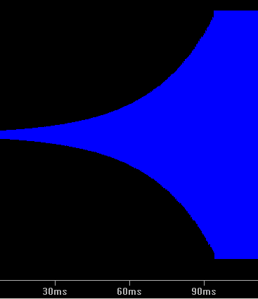
However, we can do it easier by building our circuit in Spice and running an AC analysis on it:
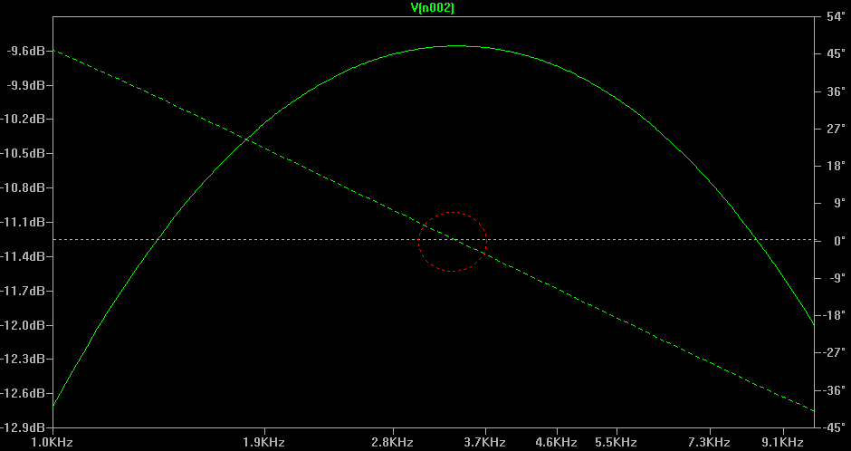
The white line corresponds to zero degrees phase and the dotted trace line crosses it in the red circle. Note that also corresponds with the maximum signal transfer. The math and the plot show the zero-phase-shift frequency is around 3.4 kHz.
But note that the gain here is about -9.6 dB — the output signal is about 1/3 of the input. We’ll need to set the amplifier gain to about three to compensate for this. (Would you like a quick refresher on decibels?) With this filter topology, it turns out that no matter what values of R and C you use, the zero-phase-shift gain is always 1/3, and the amplifier gain will always need to be greater than three.
Wait, What?
It is all well and good to just read a number off a chart, but let’s quickly derive the filter gain. You can think of R1/C1 and R2/C2 as complex impedances. At the frequency we care about, we know that the reactance of C1 (and C2) will be 4.7 kΩ. The circuit becomes a voltage divider with R1/C1 as the “top” element and R2/C2 as the bottom. Let’s call those elements Z1 and Z2.
Z1 will equal the square root of the sum of R1 squared and C1‘s reactance squared, which is really just two times 4700 squared (remember C1‘s reactance is 4700 at resonance). So Z1 is about 6.6 kΩ.
Z2 is trickier because they are in parallel. There are several ways to think about it, but I like to take the reciprocal of 4700, square that, multiply by two and then take the square root. So Z2 is about 3.3 kΩ.
A voltage divider with 6.6 kΩ at the top and 3.3 kΩ at the bottom will work out to 3.3 / (6.6+3.3) = 3.3 / 9.9 = 1/3. If you are an algebra whiz, you can work this symbolically and find out that the answer is always 1/3 as long as resistance is positive.
Amplify
 Adding a 3X amplifier is easy. In reality, you need just a little bit more gain to overcome other losses in the circuit. (See
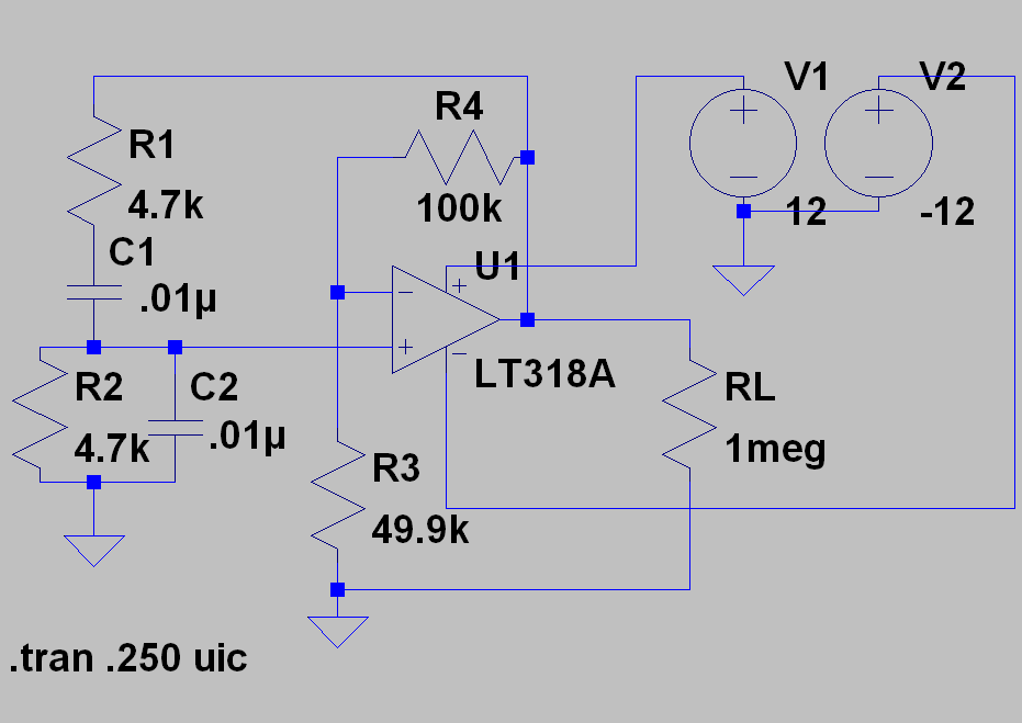
 wien-osc.asc from GitHub.)
The R1/C1/R2/C2 network is the same as before, but now there is an op amp set up as a non-inverting amplifier. The gain is set by R3 and R4. R3 should be about 50K and the gain is 1 + R4/R3 which would be 3. With the 49.9K value the gain is just a bit more. In practice, keep in mind that component tolerances and temperatures will affect values, too.
There are two things you have to be careful with to make this simulate correctly. First, you need a real op amp model that has noise so the oscillation will start. There are other ways to introduce noise, but using a practical op amp model usually does the trick.
The other thing is you need the “uic” option on the .tran simulation card. Without this, the analyzer figures out a steady initial state for the capacitors, and you won’t get oscillation. These sort of things are necessary because the simulator components are too perfect.
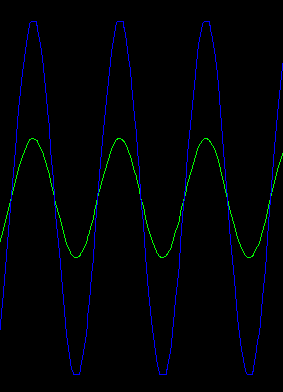 That’s interesting to see the signal start off small and get a little bigger each time through the loop until it levels out just after 90 milliseconds. However, let’s zoom in after the oscillator has started up. Notice that the green trace (the + input of the op amp) is in phase and about 1/3 of the output signal in blue. Try it and select View | FFT on the plot pane’s menu to see the output at the desired frequency and some fairly low harmonics. Because there’s no automatic gain control (see below) there is some clipping, but it isn’t very severe, because in simulation it’s pretty easy to get the gain of the amplifier nearly exactly right.
What If?
The beauty of trying this in Spice is that it is very easy to adjust parameters and see what happens. Try changing R5 to exactly 50 kΩ. Then bump it up higher. Then go a little lower. You’ll see that too much amplification results in distortion. Too little will cause the signal to die down eventually.
Many practical designs use a nonlinear device of some kind to adjust the gain dynamically. The brilliant idea that made Hewlett-Packard’s first product, the HP200A back in 1939, was to use a lightbulb as the gain adjusting circuit: as the voltage in the circuit gets higher, it heats up and the resistance increases, reducing the gain. The schematic appears in the original patent. Another common configuration uses diodes to allow gain to be higher on startup but then reduce as the signal level rises.
Try changing C1 or C2 independently. Obviously, if you change them together — or change R1 and R2 together — you’ll just adjust the frequency.
What’s Next?
If you are up for a challenge, can you replace the op amp with a FET or a bipolar transistor? Just remember the amplifier has to be in phase and have a gain greater than or equal to three at the frequency of interest, and closer to three to avoid distortion.
Because op amps are typically gain limited at higher frequencies, you don’t see the Wien bridge used much at higher frequencies. But there are many other kinds of oscillators you can try simulating. However, nearly all of them will have this structure of an amplifier with some sort of feedback. The total feedback, including the amplifier, has to be in phase and the total gain around the loop has to be one. In a simulation, it is really that simple. In practice, though, there’s a lot of gotchas like parasitic capacitance, unwanted nonlinearities, and other concerns. However, the simulation can help clear up your understanding of how things work and make the practical realization of your design as painless as possible.


“Circuit VR is where we talk about a circuit and examine how it works in simulation with LT Spice. ”
And here we was thinking VRing through a physical circuit (as exciting as that would be).
And I thought that Barkhausen was where I put das hund when he is being too vocal.
Haha!
It’s where you go, metaphorically, in Germany, when you’ve been bad. “I forgot the Valentine’s day flowers, und seit dem wohne ich in den Barkhaus.”
Hackaday: Come for the tech, stay for the multi-lingual puns.
Whoa, nice to see an article like this!
I learned from the analog “old timers” in my first job about how hard it is to make oscillators. The saying was “oscillators won’t;
amplifiers will!” (Translation: Especially at high frequencies, try to design an amplifier and it will oscillate, and try to design an oscillator and it will definitely not work!)
Great article!
That’s why a good design rule of thumb is to always use inverting amplifiers, because the feedback through any miller effect will be negative.
Then you get the opposite effect where your oscillators will only amplify while your amplifiers won’t.
Use the state variable topology – 2 or 3 opamps. Set the gain at the “right” amount to oscillate. Control the gain with a VCA (That corp?). Make the adjustment for the gain from both the sin and cos outputs (See Dave Blackmer’s RMS patent – he’s the db of dbx). sin^2+cos^2=1 You can go down to extremely low frequencies with no ripple.
You should be able to do 0.01% distortion without issue. From 0.1Hz to 100kHz.
It would be an elaborate LTspice simulation, but I’ll try and get to it sometime.
“A circuit with amplification that gets the same amount”, should be -some- amount?
No, same. Meaning the loop gain is 1.
“The Wien bridge oscillator, a very simple design that originated as a way to measure impedance back in 1891”
What did an amplifier look like in 1891?
They didn’t have good amplifiers back then. That’s part of what made Bill Hewlett’s 1939 master’s thesis so interesting.
Hewlett combined Wein’s frequency-sensitive network with Howard Black’s 1925 patent for negative feedback networks and Harry Nyquist’s 1932 paper “Regeneration Theory” (a predecessor to the Barkhausen critera) to design a high-purity sinewave oscillator. He also proved that an oscillator with enough gain to start would eventually go into overdrive and clip the sine wave down to a square wave.
The solution was to add a nonlinear feedback circuit that would reduce the amplifier’s gain as the output amplitude increased. A strongly nonlinear element would just produce clipping at a lower voltage, so he needed something whose value was nonlinear but changed gradually.
He chose the tungsten filament of a light bulb, which has a positive tempco. Running the sine wave through the filament produced heat proportional to the RMS voltage of the sine wave, the heat made the filament’s resistance increase, and putting the filament in a voltage divider gave Hewlett a well-behaved gain control element.
If rather slow-settling one. Then again, the Wien bridge isn’t easily adjusted anyhow because you have to change multiple component values simultaneously and tracking between two potentiometers or variable capacitors is never perfect.
As a software only guy, I am always impressed, and somewhat jelly of all you amazing people who understand and work with analog.
HaD Said: “There are two things you have to be careful with to make this simulate correctly. First, you need a real op amp model that has noise so the oscillation will start. There are other ways to introduce noise, but using a practical op amp model usually does the trick. The other thing is you need the “uic” option on the .tran simulation card. Without this, the analyzer figures out a steady initial state for the capacitors, and you won’t get oscillation. These sort of things are necessary because the simulator components are too perfect.”
In SPICE circuit development/simulation (LTspice for example) setting the uic directive (skip initial operating point solution) is often NOT the best way to “kick-start” an oscillator like used in this example.
Often a better way (at least in early development) is to set an Initial Condition (.ic SPICE directive) on a carefully selected (critical) node and let the simulation run as normal (without the uic directive option).
Not using uic will also you to use (for this Wien example) an “ideal” Op-Amp model, or even a custom behavioral circuit or subcircuit, with or without a noise source.
Relying on a “real” op amp model that (supposedly) has “noise” so the oscillation will start (as stated in the article) is NEVER a guarantee the circuit using a real physical Op-Amp simulation model will work on the bench. But using the .ic directive in simulation at the design stage will allow you to understand which circuit nodes are critical to induce (or NOT induce) oscillation.
Not using the uic option will allow you to see how the solver converges to the stead-state operating point (look at the SPICE Error-Log).
Using the uic option will often result in start-up transients being saved that can corrupt what you really want to see in the Waveform Viewer plot (unless you fight with customizing the display to remove the auto-scale plots). In this particular simulation example with uic enabled you an see the Op-Amp output at startup has a big +/-10V transient. That’s OK for this particular simulation, but this WILL be a problem with most other circuits, especially circuits with a single-rail power supply. Of-course you can always eliminate startup transients by saving data later in the simulation time, but we’re more interested in startup behavior in this case.
Finally, by not using the uic option and carefully controlling the initial condition node directive(s), you should be able to reduce the simulation time required to see what is going on in the development phase.
As a quick and dirty example: In the “wien-osc.asc” LTspice simulation schematic downloaded from GitHub as linked in the HaD article, do the following:
1. Right-click the directive “.tran .250 uic” and UNCHECK the “Skip Initial operating point solution” box.
2. Left-click Edit > Spice Directive and in the pop-up box type the following:
.ic V(n005)=1
Now click OK and place the directive line anywhere in an open space on the schematic.
3. Run the simulation. Now when you click the Op-Amp output in the Waveform Viewer window, you will see the oscillator start-up from the initial condition set at V(n005) by the .ic directive above.
4. Now that the simulation reaches steady-state faster with the .ic directive and no uic, you may significantly reduce the simulation data save time in the .tran directive (Right-Click it). Try Stop Time: 50 instead of 250. Now the simulation reaches steady-state 5-times faster.
5. When the simulation is done, look at the SPICE Error-Log. Now because uic is turned off, you can see the operating point convergence results.
Keep in-mind, there are times when using the uic option is good and times when it is bad. Try both methods in different stages of your design.
You can always turn-off the .ic directive in the schematic window by Right-Clicking it and setting it to a Comment. Then Right-Click the .tran directive and turn uic on again.
Suggestions to the Author of the example “wien-osc.asc” LTspice simulation schematic downloaded from GitHub:
* Please include the accompanying .plt Waveform Viewer plotter file along with the .asc Schematic file when you publish an example simulation. Also include the .log file as well if the Error-Log output is relevant to the simulation.
* Label the nodes you show in your .plt Waveform Viewer file. It makes documenting the simulation MUCH easier. Just click the “Label Net” icon in LTspice.
Have Fun :-)
Typo: “Not using uic will also [allow] you to use (for this Wien example) an “ideal” Op-Amp model, or even a custom behavioral circuit or subcircuit, with or without a noise source.”
Thanks for the detailed notes. I’ve used .ic, but I wanted to keep this simple for brevity as it is not always obvious in some circuits where to put the initial condition.
Great tip about labeling plots. Most of my Spice was on punch cards and I knew how to label nets but didn’t know you could label the plot traces. Great tip.
“Inverting a signal is equivalent to adding a 180-degree phase shift, ”
In case of oscillators, sin-Cos waves, square waves, true
But, in case of rectangular waves, not true. Whenever I am explaining something to my friends/students, and I say ‘inverted’ , everyone just conveniently assumes that it means 180⁰ phase shift. Which is not true for rectangular or continuously modulated PWM wave.
How do you delete this symlink of “180⁰ shift is inversion” from minds of everyone around you?
Even, many of my teachers think the same. What the f*** you think from symmetric wave perspective every time ?
However, very great article otherwise.
weren’t incandescent lightbulbs used in wein-bridge oscillators for some reason at some point??
https://cdn.hackaday.io/images/3605721464296374306.png
Does that qualify ?
source : https://hackaday.io/project/9376-yet-another-discrete-clock/log/38746-success-a-minimalist-single-mosfet-quartz-oscillator
P-DOG, The Hewlett design innovation *IS* the reason that these oscillators used incandescent bulbs and its still found in designs today. It was also the basis for their first product and what made that product unique and desirable.