Don’t get me wrong. Like most people, there’s nothing I enjoy more than solving a long, involved math problem by hand. But, sometimes, a few pages of algebraic scratches on paper is just a means to an end. I find this especially true during electronic design sessions, be it circuit design or PCB layout; I just need the answer, and any time spent finding it distracts me from the larger task at hand. For me, at least, this seems to happen at least once a week, and about five years ago I decided to do something about it. I had heard of computer algebra packages, of course, but they weren’t taught as part of the undergraduate engineering curriculum when I went to school. So, I set about learning one: let the computers do the math!
The package I chose is wxMaxima, a document-based front-end to the Maxima computer-algebra system. Descended from code originally written in the late 1960s, it’s a general-purpose package supporting symbolic computation for algebra and calculus. There’s solid, mature code underneath with a modern UI veneer on top. Plus, it’s FOSS.
As I’ve progressed, I’ve found that some additional functions make the Maxima environment especially convenient for circuit design. A few are simple enough that I’d typically just re-create them as needed, so I never really got organized – there were several versions of my “library” floating around on various machines. I finally got my act together, cleaned up the most-frequently used functions, and put them into a GitHub repo.
Let’s have a look at how we can use them to take the tedium out of math for some design problems.
Preliminaries
There are few things we need to know about Maxima syntax, which differs from the usual languages you may be more familiar with:
- Lines are terminated either with a semicolon, which shows the resulting output, or a dollar sign, which suppresses it.
- Variable assignment uses a colon. To set variable “x” to value “3,” we say “x : 3;”.
- The equals sign establishes a symbolic equality relationship: “y = 2*x;” defines an equation that can be manipulated symbolically.
- If you mix up #2 and #3, you’ll get very confused.
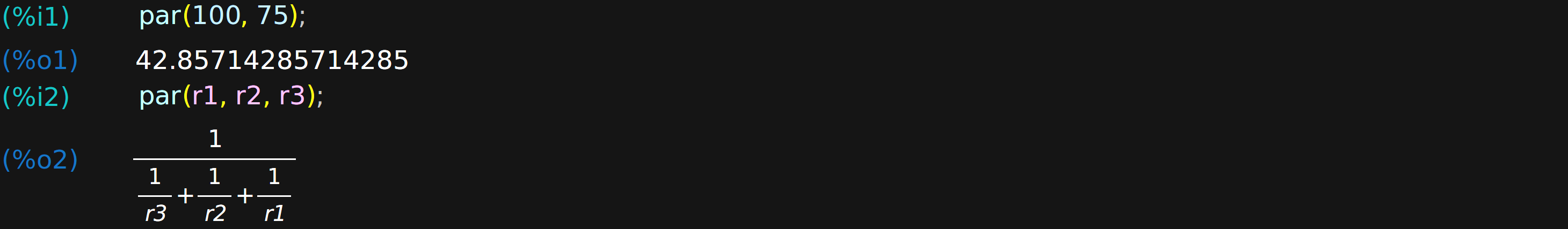
With these in mind, we’re prepared to have a look at some functions from the GitHub code. Three simple functions end up being very useful. The first function, par(), calculates equivalent values for parallel resistors or inductors, or for series capacitors. For example:
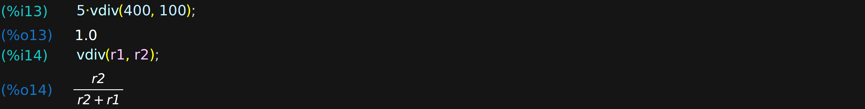
The second function, vdiv(r_top, r_bot), calculates a voltage divider ratio for the given resistors. In the first example, a 5 V supply is divided by 400 and 100 ohm resistors to yield a 1 V output, while the second example creates a symbolic expression for the divider formed by r1 and r2.
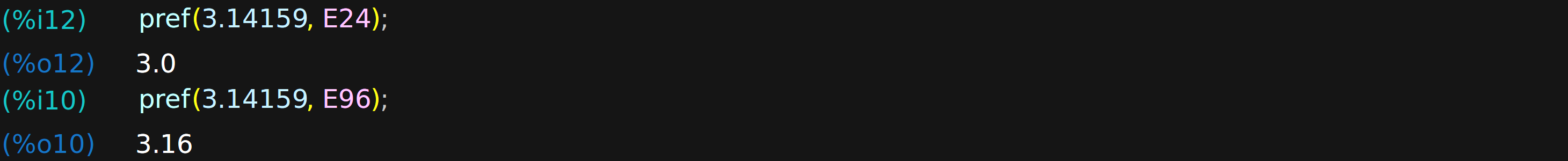
Finally, the pref(x, E) function finds the closest value to x from the selected EIA “E-series” of preferred values. You can choose any series from {E3, E6, E12, E24, E48, E96, E192} plus the combined series {E48_E24, E96_E24, E192_E24}. For example, we can find the closest 5% and 1% resistors for a value of approximately pi ohms.
Armed with these three functions plus the built-in power of Maxima, we’re ready to tackle some problems.
VGA Output: The New Blinking LED
 Since 2019 is destined to be the year that hackers fully embrace the power of FPGAs, it seems only fitting to apply these techniques to a common FPGA example. While the introductory microcontroller project is traditionally the blinking LED, simple VGA output is the first “real” FPGA project for many. To generate the analog signals, a few digital output lines are typically fed into a simple resistor-based DAC per color channel, with sync lines handled by two other outputs.
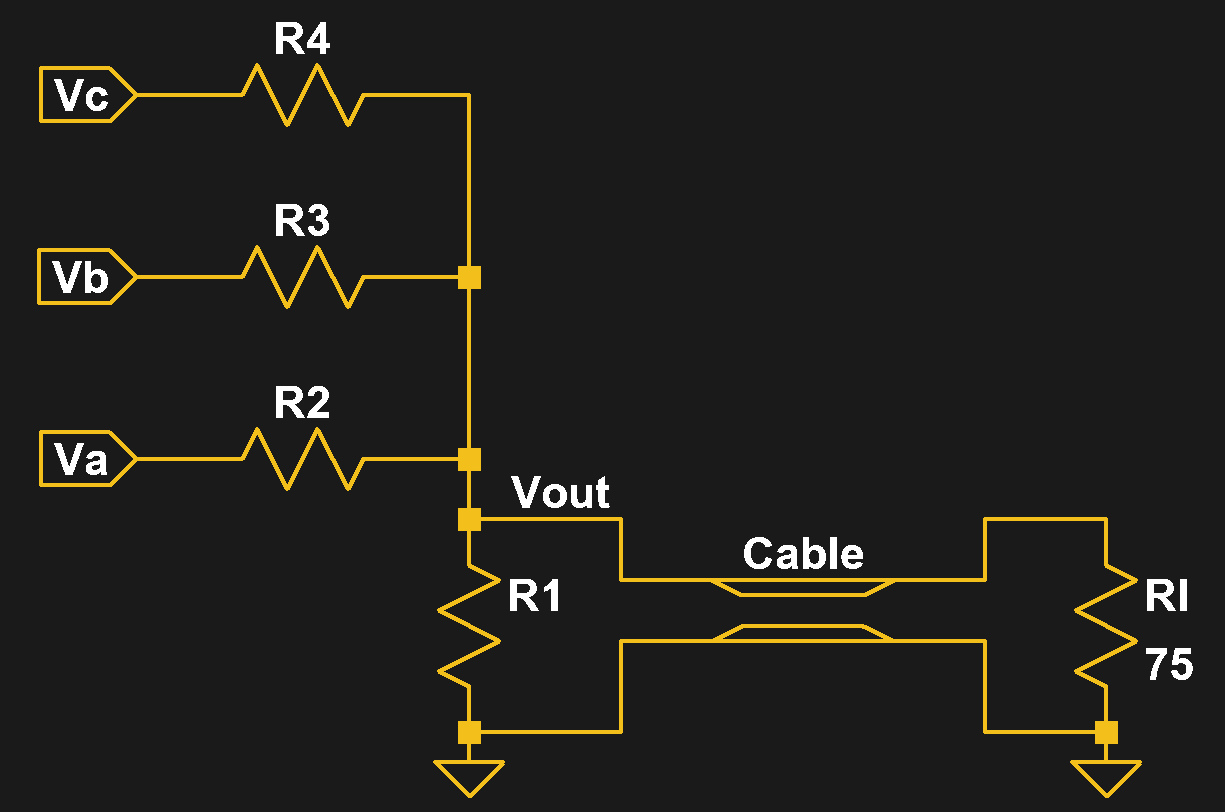
The circuit shown here represents one color channel (say, red), and allows for eight distinct output levels from three bits of input, so the RGB display will be capable of 512 colors. In this case, Vc is the MSB, and Va the LSB. This topology is a simple weighted-resistor DAC, and we choose it over the more common R-2R variety because the latter (pun intended) requires seven resistors instead of four. There are a few things we know right away, namely that our supply voltage is 3.3 V, while the full-scale output (Vmax) for the DAC should be 0.7 V when loaded with the 75-ohm terminator (Rl) inside the monitor (we know this from the VGA spec).
![]()
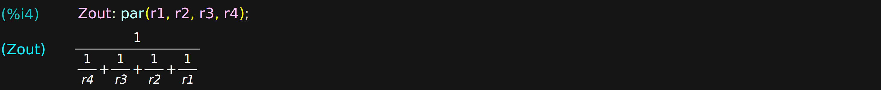
We need to find the values of four resistors (R1 – R4), so we’ll need to come up with four equations to solve. One of them should set the output impedance to 75 ohms to avoid reflections on the cable and the resulting blurriness on the display. From the schematic, we see that the output impedance is simply all the resistors in parallel (imagine Va, Vb, and Vc all connected to ground). So, we define a variable, Zout, using the par() function. Later, we’ll create an equation assigning it the value of 75 ohms. The result we get back shows a nicely formatted version of the formula:
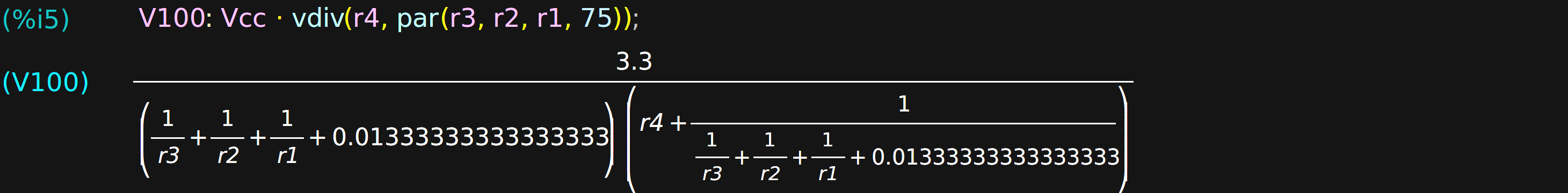
We need three more equations. There are a number of sets that one might choose, but maybe the simplest way is to consider the output voltage when only one of the input lines is in the high state. For instance, when just the MSB is high – the state {Vc=1, Vb=0, Va=0}, or “100” – the resistors form a voltage divider from Vcc with R4 as the top resistor, and all the others in parallel as the bottom resistor. We use the vdiv() and par() functions to define a variable V100 for this state, which we’ll also create a subsequent equation for. The output is a messy expression to us, but Maxima isn’t bothered by it.
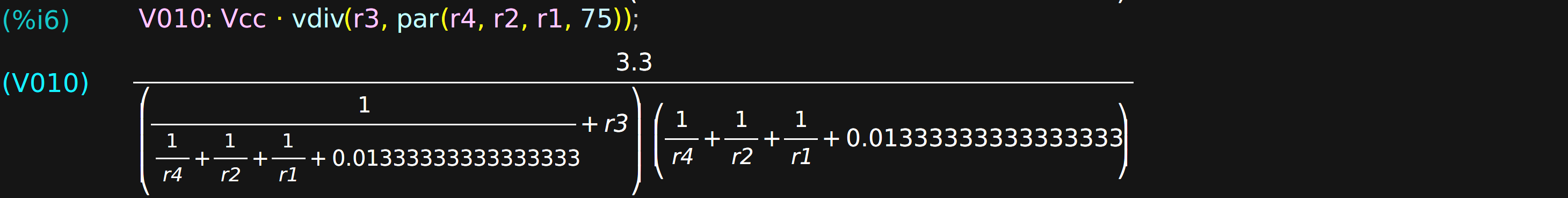
Similarly, when only Vb is high (the “010” state), we can define V010 with a similar voltage divider, this time with r3 as the top resistor, and all the others paralleled on the bottom.
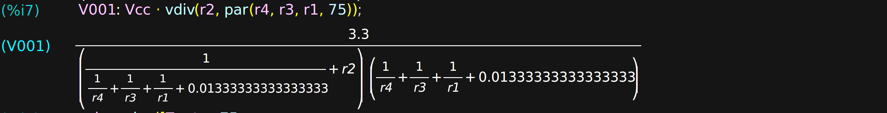
Finally, applying the same logic to the “001” state yields an expression for V001.
Now, we can form the four equations and have maxima solve() them. The first equation sets the output impedance to 75 ohms, while the remaining three set the voltage outputs for the states we’ve chosen. For a 3-bit DAC, the MSB has a weight of 4/7 of the full-scale voltage, the middle bit has a 2/7 weight, and the LSB a 1/7 weight. Equating the three voltage states with these fractions of Vmax gives us the other three equations. Along with the equations, we also pass a list of variables to solve for: the resistor values.
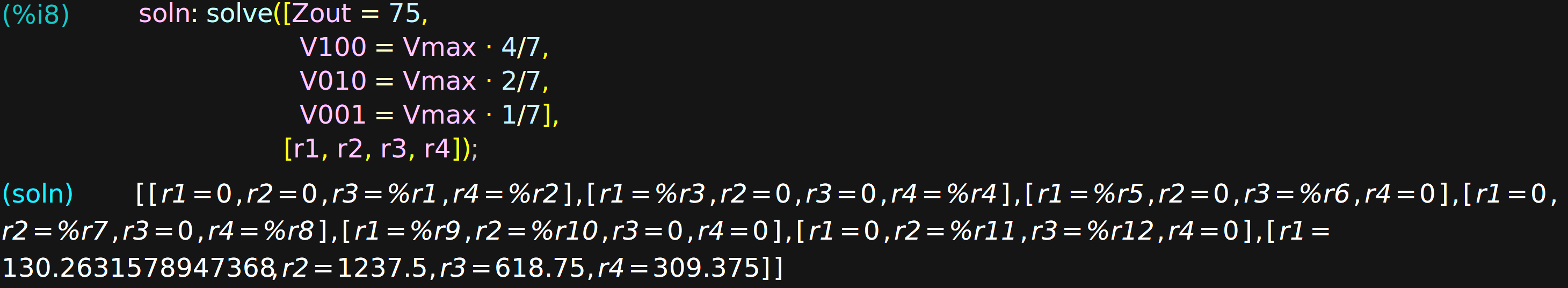
The output shows two things: our desired solution, and the fact that the output of computer algebra packages can be messy. In this case, the way the problem has been solved has introduced a number of “solution” families that we don’t particularly care about. The last one in the list, however, is obviously what we’re looking for.
Since we’re not likely to buy a 130.26316-ohm resistor, we can select the closest values from the E24 (5%) series and assign the result to the variable “vals.”
![]()
Of course, selecting these values will change the performance of the DAC, so it’s best to check what these resistors actually produce. The ev() function evaluates its first argument using the context of the second, so in this case, we’re substituting the preferred value resistors. (The fpprintprec variable controls the floating point printing precision; here it has been set to four significant figures.)

The outputs should ideally be [75, 0.4, 0.2, 0.1]. I’d probably be OK with these values, maybe because I have a large stock of 5% resistors, but if we wanted a closer result, we could simply find the preferred values from the E96 (1%) series instead.
There are a couple of footnotes to this analysis. First, we’ve ignored any output impedance for the drivers into the DAC. If we know their output impedance (or can measure, guess, or deduce it from graphs in the datasheet), we can subtract it from each input resistor to compensate. We’ve also conveniently left out gamma correction, which unfortunately can’t be done with just a resistor network. Finally, this is just one way to calculate the resistor values. You could instead use the knowledge that R1, R2, and R3 should be related by factors of two to simplify the calculations, although maybe the point is that you don’t have to be so clever.
555 Timer Servo Controller
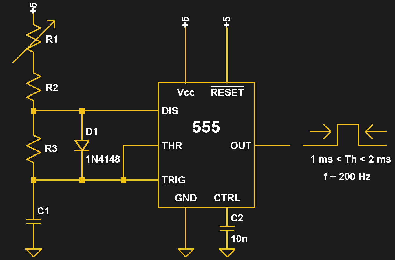 As a second example, consider the design of a servo controller using the ubiquitous 555 timer IC. Let’s say we have a 10 k potentiometer (R1), and we want to control the servo position with it. We need the 555 timer to output pulses between 1 ms and 2 ms, corresponding to the full travel of the servo, as the potentiometer travels its range. We also decide that the pulse repetition rate should be 200 Hz or lower. Consulting the Wikipedia page, we find that the addition of a diode to the typical 555 astable circuit lets us have duty cycles less than 50%, which we need to generate the pulses. The page also gives us equations for the high time (Th) and low time (Tl) with the added diode.
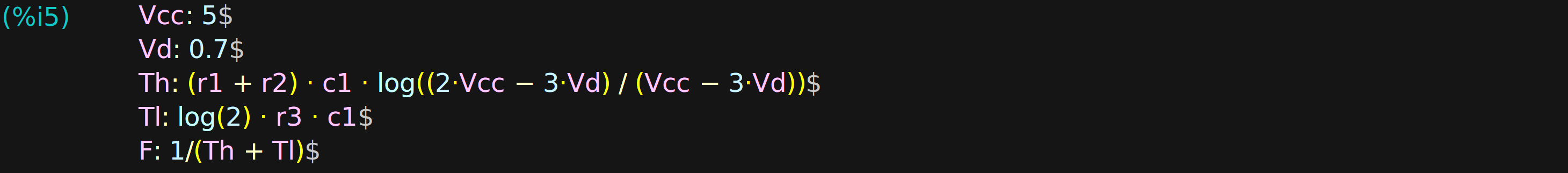
To start the design, we dump everything we know into variables. We choose a 5 V supply for Vcc, and assume a forward voltage of 0.7 V for the diode (which we’ll revisit later). The expressions for the high time (Th) and low time (Tl) are direct translations of the equations given on the Wikipedia page, while the frequency (F) is simply the reciprocal of the period.
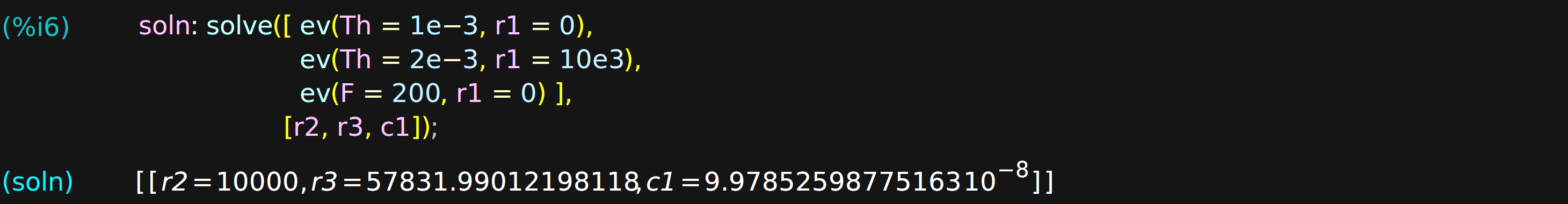
Given these definitions, we can now write three equations to constrain the solution for the three unknowns, r2, r3, and c1. We use the ev() function, which evaluates expressions given a list of relationships. For instance, the first equation, “ev( Th = 1e-3, r1 = 0 ),” says that the pulse width should be 1 ms when R1 is set to zero (rotated all the way to the left). Likewise, we set the pulse width to 2 ms with R1 set to its maximum resistance (10k). Finally, the last equation says that the frequency should be 200 Hz with R1 at zero. These three equations are enough to solve for the three unknowns.
Again, the results are not all values we’re likely to find in the junk box, so we can choose the closest 5% values.
![]()
So, we can check our parts stash for 10k and 56k resistors plus a 100n capacitor. If we wanted to be cautious, we could also check that these substitutions haven’t substantially changed the solution by evaluating the pulse width and frequency with R1 at both extremes.
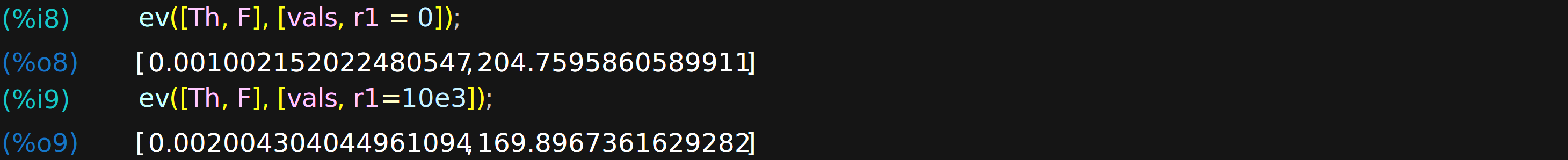
The results look good: 1 ms to 2 ms pulses at between 170 Hz and 205 Hz. But, of course, this only validates that the chosen components work with the circuit model we’ve chosen. Underlying this model is the assumption that the diode forward voltage is a known constant 0.7 V. In reality, this forward voltage varies with the current through the diode: a quick peek at the 1N4148 datasheet shows that it’s probably around 0.5 V at the currents involved in this circuit. So, before building the circuit, we might want to re-run the calculations using this value. Either way, the results get us in the ballpark and ready for the next step, whether that’s simulation or prototyping.
PCB Footprint Conversion
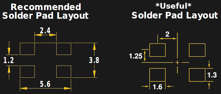
Here’s a final simple example that I frequently use for creating PCB footprints. In Eagle, footprints are created by placing pads of a specified size at a specified center point. Some datasheets give their footprints in this format, while others force you to do some math to convert the dimensions. I used to do these in my head, but after receiving a trio of purple coaster PCBs due to a stupid mistake, I make my computer do the work now. Two quick equations can be found by inspection, and maxima does the rest. In this case, I express the dimensions the datasheet gives in terms of what I want: the size (h, w) and position (x, y) of the pads.
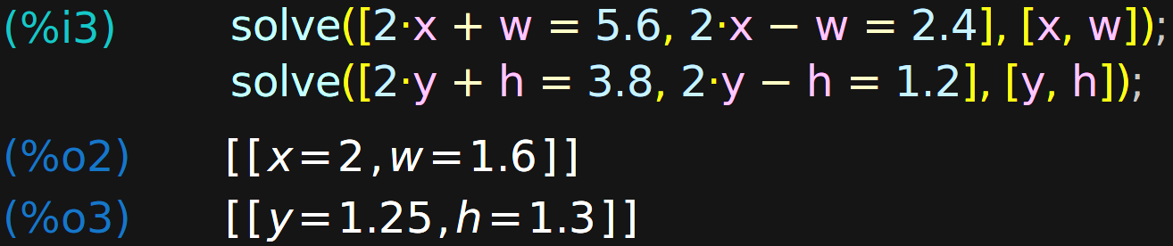
Typing in the equations only takes a few seconds, and greatly reduces the probability of a stupid mistake relative to doing the calculations manually.
Going Further
If you’re intrigued by Maxima and want to get started on your own, there are many tutorial links on the github.io page. There also a number of examples on the web specific to circuit design: an analysis of damping in oscillators, some introductory circuit analysis, applying differential equations to RC circuits, and transistor amplifier design (PDF warning).
Of course, computer algebra isn’t the only way to solve circuit problems. You could also use a good-old spreadsheet.


Another article about generating video signals with correct amplitude and output impedance
https://hackaday.io/project/148298-32-shades-of-grey
http://danjovic.blogspot.com/2015/02/gerando-sinais-de-video-num-pic-com.html
In practice as the number of bits gets higher the resistor tolerances get more and more critical
Yes.
Maxima is my favorite tool to solve such problems when I’m in a hurry or when the problem is just too big to be solved by hand.
Highly recommended.
Funny, just uploaded a maxima script to generate equation system from a netlist:
https://github.com/danselmi/sycira/blob/master/sycira.mac
(tools to convert spice netöist will follow)
Awesome stuff. I thought about this a few times, and started down the KCL/KVL analysis route, but didn’t get very far. You’re either going to have an amazingly useful tool or a way to bring Maxima to its knees instantly :-) I’m excited to see how it turns out.
My preference is usually to avoid learning a new special purpose language for everything, so instead tend to turn to the SymPy package and leverage all the things I already know how to do in python.
I thought macsyma was built on MIT Scheme. Which would be general purpose. Is that not true?
Maxima is wonderful stuff.
You didn’t mention that it does bignums, actual rational numbers, and symbolic calculus as well…
(%i8) integrate(1/x, x);
(%o8) log(x)
Back when Mathematica was brand new (for the NeXT computer), there was a book out called “Mathematica for the Sciences”, which showed what you can do with a symbolic mathematics package. One of the chapters on electronic circuits showed how a simple resistor-and-diode was nonlinear and unsolvable, and that the diode forward-bias voltage was a simplification to the actual situation which could be simulated. It was a revelation to read compared to the usual simple cookbook formulas in the usual electronics books at the time.
(Of course, Mathematica was and is horribly expensive for an amateur like me, so I spent a good part of the 90’s looking for some alternative for my Windows 3.1/95 machine. I ended up using REDUCE, which even though would crash on bigger problems at least had reasonably useful demo versions for free. I could convert programs from that book, which I checked out from the library constantly. Didn’t find Maxima till much later, and then didn’t want to switch.)
Mathematica is 300$ or so for the individual nowadays (home edition)
Free on a rpi.
Interesting – could be helpful in designing attenuators.
In T or Pi format, you often need a specific resistance. Having E192 tolerance resistors helps, but I usually go for 2 [or 3] resistors in parallel, boosting the overall power handling.
Picking the right resistors sounds like just the job for this algebra app.
The example in the GitHub writeup is exactly that – designing a pi attenuator. (just scroll down a bit on the page)
https://github.com/tedyapo/maxima-circuits
I’ve wanted to make a ‘find the closest N paralleled resistors’ or similar function for a while, but never got around to it.
Layout of the components:
Thanks for these examples. Maxima is awesome. Python heads should also have a look at Python’s SymPy library that does symbolic manipulation
CAS calculators are a thing, and now often have decades that have gone into their software and usage scenarios. The HP Prime is a particularly good value, after you add the program to allow touchscreen text entry. Bench usage, of course, is a major benefit for such dedicated tools.