If you want to do something you’ve never done before, there are two broadly-defined ways of approaching it: either you learn everything you can about it and try to do it right the first time, or you get in there and get your hands dirty, and work out the details along the way. There’s a lot to be said for living life by the seat of your pants. Just ask anyone who found inspiration in the 11th hour of a deadline, simply because they had no other choice.
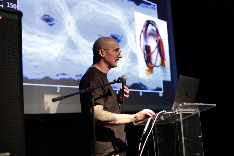
Ted Yapo didn’t have a lot of high-speed design knowledge when he set out to build an open-source multi-GHz sampling oscilloscope, but he didn’t let that stop him. Fast forward a year or so, and Ted’s ready to build his third prototype armed with all the hands-on practical knowledge he’s gained from building the first two.
At the 2019 Hackaday Superconference, Ted gave a talk about his journey into the high-stakes world of high-speed design. It’s an inspiring talk, and Ted gives a good look into everything he’s learned in trying to build a sampling ‘scope. We think you’ll appreciate not only Ted’s work, but also the ease with which he explains it all.
So why is Ted doing all of this? For one thing, his 1989 Tektronix has been trucking along for 75,000+ hours, and it won’t last forever. The bigger problem is that this is one of the last digital scopes to use equivalent-time sampling, because manufacturers jumped to real-time sampling within a few years. Ted sees the opportunity to duplicate this with modern technology, and we are over here nodding vigorously and setting aside cash for whenever this thing is ready to either buy outright or build.
Equivalent-Time Sampling
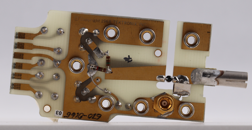 The first scope Ted ever used was a 1968 Tektronix, so that’s where he started his studies. His journey began with that age-old question: how do equivalent-time sampling ‘scopes work, exactly? He found schematics and descriptions for that vintage, and then bought a used one and dismantled it.
What Ted found inside the sampling head seems shockingly simple. There are two Schottky diodes doing the sampling, and they are fed short current pulses by a separate strobing circuit controlled by a step recovery diode.
Ted quickly discovered that the biggest hurdle would be generating these extremely fast pulses. He found that while it’s harder for the hobbyist to get bleeding-edge components that get the speed down to single-digit picosecond range, it’s definitely possible to get to the 20-30 ps range with affordable components.
 Analog to Digital Conversion
Armed with enough knowledge to be dangerous, Ted built an analog sampler using a six-Schottky diode gate and a couple of 74HC logic chips to generate the strobing pulses. Ted says it took half an hour to take his first sample because the UI is completely manual — he sampled using a potentiometer, read the values off of a voltmeter, and wrote them all down, covering five sheets of paper. But it worked, and he calculated the bandwidth at 141MHz.
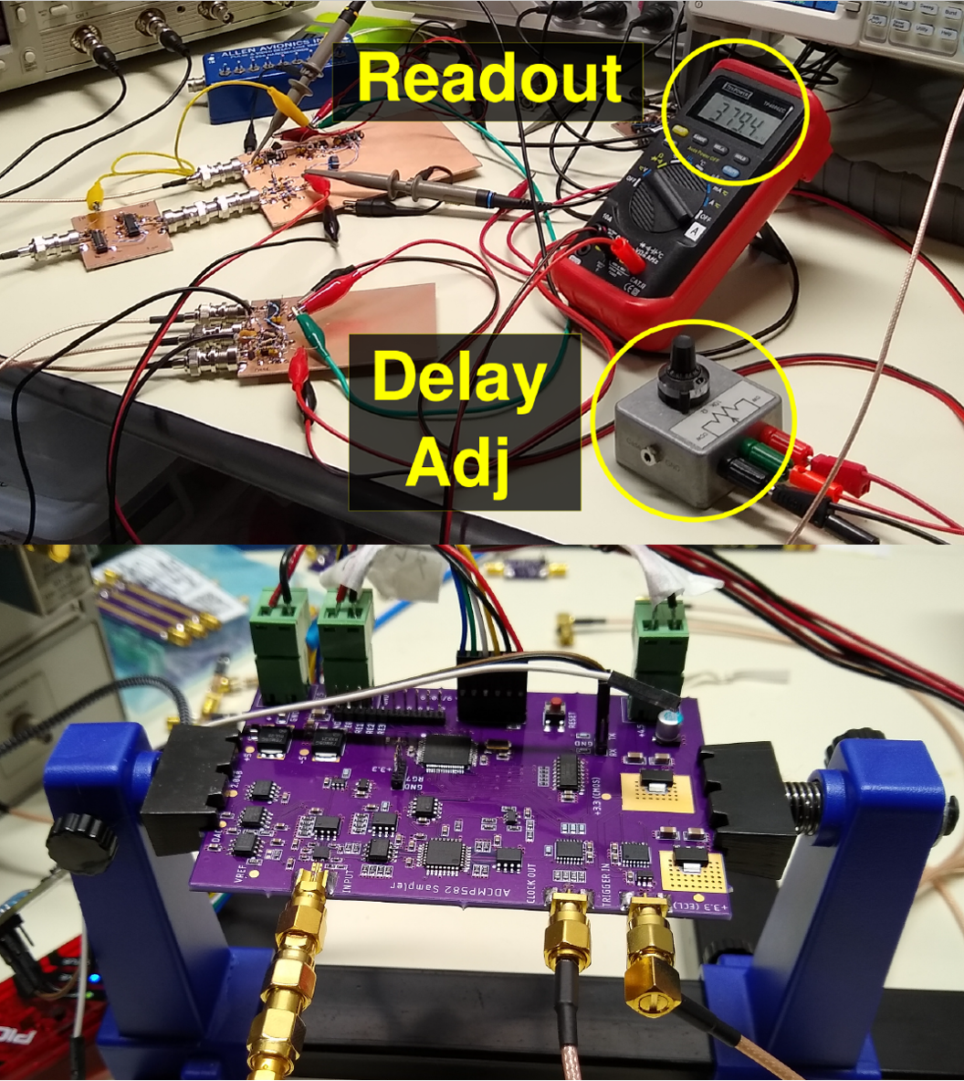
For his second prototype, Ted went digital. He explains that this method uses a comparator: it compares two inputs, and tells if one is higher than the other using successive approximation. This is the sampling part. But you also need a time base, and he ended up using a switched gate delay to align the clock edges.
Ted’s second prototype is several orders of magnitude faster than the first. He’s up to 7GHz bandwidth, has the rise time down to 48 picoseconds, and averages 100 gigasamples per second. Amazingly enough, the BOM comes in under $100 including the PCB. Are you salivating yet?
 Fast Signals For a Fast ‘Scope

So, what can you do with such a fast scope? One thing Ted wants to do is Time Domain Reflectometry (TDR), which is a lot like radar for transmission lines. By sending a signal down a PCB trace or wire and measuring what comes back, you can determine the characteristic impedance of a circuit or section of a circuit.
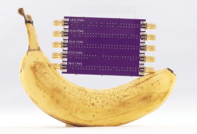
Ted talks about a common problem in high-speed circuit designs: calculating the right trace width necessary for a coplanar waveguide. In other words, how wide should the copper squiggle connecting the components be to achieve standard 50Ω impedance? Many calculators have been built to make this easier, but they’re all based firmly in theory that doesn’t account for the realities of uneven impedance across the fiberglass in PCBs. So Ted made a board to test different trace widths. None of them hit 50Ω exactly, but with his handy new 7GHz ‘scope, he was able to easily determine that 22mil traces are optimal given the circumstances.
For the third prototype, Ted is shopping around for a 32-bit CPU and a way to enhance the time base circuitry. Aside from ultra-wideband radar and LIDAR, Ted is looking for interesting use cases, so hit him up on IO or Twitter if you’ve got fast signals that need scoping out.


Looks alike to Walter White, I will be cautious with questions when conference ends ……… ;)
More like Mahatma Gandi!
Wow. He nailed this, both in experimentation and explanation. Kudos.
I have to say, Ted’s approach to design reminds me of how I used to go at things. Build to learn, piece by piece, then put the puzzle together. Thanks for sharing Ted.
This is a great talk. Does anyone have any links to the background of what he’s talking about? Such as the schottky sampling?
Some time ago I found this project that explains the principles in details.
http://www.redrok.com/sampscope.htm
Seems more of a link for building a sampling front end with some explanation of the specific parts used, rather than explaining anything about the underlying theory behind it.
The schottky is used as a very fast switch to take a snapshot of the input signal.
FYI: https://www.digikey.com/en/articles/techzone/2016/dec/how-and-why-to-use-pin-diodes-for-rf-switching
A PIN diode is a special form of diodes that are good for switching very fast.
I’m afraid that’s incorrect: PIN diodes are bad at switching quickly.
Silicon diodes can’t shut off instantly because there are charge carriers in their depletion region while they’re forward biased and conducting current. If you reverse the voltage across one quickly, current will flow through it backwards (the direction it shouldn’t go) for a short time until all the carriers are flushed out of the depletion region.
PIN diodes have an extra layer of ‘intrinsic’ (undoped) silicon between their P and N layers, which stores extra charge carriers. The lifetime of the stored carriers is long enough that a PIN diode will conduct current both directions with little distortion for frequencies above a few megahertz.
PIN diode switches for RF applications work by changing the voltage of the signal so it can or can’t forward bias the diode in the first place. The amplitude of the RF signal is much smaller than the bias voltage, so adding or subtracting 500mV is enough to make the PIN diode look like an open circuit or a short circuit to RF signals.
Schottky diodes don’t have the kind of depletion region silicon diodes have. They work based on the relative energy levels of electrons in the conduction band of a piece of metal and the conduction band of a piece of doped silicon.
If electrons in the silicon’s conduction band have more energy than electrons in the metal, it’s easy for them to move from the silicon to the metal, but hard for them to move from the metal to the silicon. That difference in energy levels is called a Schottky barrier, and Schottky diodes are also known as ‘hot carrier diodes’ because only the electrons with the most energy from thermal vibration (the hottest ones) can cross the barrier. By applying an external electric field, you can make it easier or harder for electrons to move across the barrier.
Since Schottky diodes don’t store charge carriers in a depletion region, they can shut off almost instantly. That makes them useful in switches that have to turn on and off quickly (as in ‘picoseconds’ quickly).
The usual switch for a sampling oscilloscope is called a diode bridge: you put two pairs of diodes in parallel, oriented so they’re all either forward biased at the same time or reverse biased at the same time. Then you put the diode bridge between a pair of resistors, and you put the resistors in an H-bridge. When the bridge switches one way (the ‘on’ state), all of the diodes conduct. When the bridge switches the other way (the ‘off’ state), all of the diodes are reverse biased.
Assuming the diodes are matched, they’ll all have the same forward voltage when the H-bridge is in the on position. If you connect an input signal to the middle of the bridge’s left side, the voltage at the middle of the bridge’s right side will rise and fall to match it. In the off state, the diodes are reevrse biaed and the voltages on either side of the bridge are pretty much independent of each other.
The sampling switch works by keeping the H-bridge in the off state most of the time, and snapping it into the on state with a train of short pulses.
The fast turn-on and turn-off times of Schottky diodes make it possible for a diode bridge to match the input and output voltages and then shut off again for pulses a few tens of picoseconds wide. If the output side charges a capacitor, you get a sample-and-hold circuit that captures a snapshot of a very narrow slice of the input signal.
That’s what sampling scopes do.
Excellent description!
thanks!
https://www.davmar.org/TE/TekConcepts/TekSamplingCircuits.pdf
https://www.ece.ucsb.edu/Faculty/rodwell/publications_and_presentations/theses/Allen_thesis.pdf
https://archive.org/details/schottkydiodebri1121perr/mode/2up
http://w140.com/tekwiki/wiki/S-4 and http://w140.com/tek_S4_1985.pdf and http://w140.com/frye_s4_gate.pdf
a real treasure trove, many thanks!
Tek still sells a sampling scope, but it is *not* cheap. However, it has >70 GHz BW with the appropriate heads.
https://www.tek.com/oscilloscope/dsa8300-sampling-oscilloscope
Very nice talk and *very* interesting project.
You can get a similar product from Agilent with >100GHz of bandwidth in the DCA-X, and lecroy will sell you a genuine (non-sampling) oscillscope with 100GHz of bandwidth in the UXR series for just under $1M with the edu discount.
When $1M is the “discount” price, it makes it worth founding your own university.
Quite impressive.
I’m not very knowledgable about high speed design, but as a hobbyist I browse a bit around the web and pick up some stuff.
When the weave of the glass fibre becomes an issue in impedance mismatch, there are a bunch of (more or less expensive) options. The cheapest option to improve performance is to simply not use horizontal and vertical traces for your high speed signals. Using an angle between 20 and 30 degrees seems to be most use to get a bit more performance out of FR4.
Eagle projects can be directly imported into KiCad. The import is not perfect, but often you’ll get 90% of the way in 10 minutes or so.
yeh its a good idea, if you keep everything analogue when its in the highspeed critical sampling area, then go through the digital convert after, theres no need for the high speed ADC’s anymore!
Shut up and take my money
;-)