Gravity can be a difficult thing to simulate effectively on a traditional CPU. The amount of calculation required increases exponentially with the number of particles in the simulation. This is an application perfect for parallel processing.
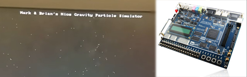
For their final project in ECE5760 at Cornell, [Mark Eiding] and [Brian Curless] decided to use an FPGA to rapidly process gravitational calculations. This allows them to simulate a thousand particles at up to 10 frames per second. With every particle having an attraction to every other, this works out to an astonishing 1 million inverse-square calculations per frame!
The team used an Altera DE2-115 development board to build the project. General operation is run by a Nios II processor, which handles the VGA display, loads initial conditions and controls memory. The FPGA is used as an accelerator for the gravity calculations, and lends the additional benefit of requiring less memory access operations as it runs all operations in parallel.
This project is a great example of how FPGAs can be used to create serious processing muscle for massively parallel tasks. Check out this great article on sorting with FPGAs that delves deeper into the subject. Video after the break.
[Thanks to Bruce Land for the tip]


Nitpickery: Unless I’m missing something, the number of calculations only increases as the square of the number of items in the simulation (not exponentially).
Yup, N^2 comparisons. In some simulations, they have been able to reduce the amount of comparisons by ignoring the attraction between very distant objects, as it would mostly negligible. Mostly.
There exist algorithms that achieve O(n lg n). See Barnes-Hut and Fast Multipole Methods. These are part of standard splash parallel processing benchmarks. So if you use a better O(n lg n) algorithm and parallelism, you can do even better.
Why does the big mass in the lower left side seems to disappear (or explode maybe?) at second 00:13?
It was attracted towards the one in the middle, and when they got close enough, they flung themselves out of view.
Seems to have the same problem my sims had, in that when things get very close the simulation sort of explodes, particles can escape with a much larger velocity than they came in with, and conservation laws go out the window. Making the iteration time step really small helped at the expense of making things grindingly slow, but nothing properly solved it. I wondered if I should be integrating along a path length or doing some sort of explicit energy or momentum accountancy. All I did was sum forces, resolve and the for each dimension do f=ma and then v’ = v + delta t * a.
How did you integrate? Newton-Feynman half step? Runge-Kutta? Predictor-corrector with Runge-Kutta might do ya better. (Note: Derivation of 4th order Runge Kutta in Numerical Recipes is wrong, but the algorithm is right. Same error in older books, so it was a copy/paste, which is too common in some kind of reference texts.)
x’ = x + v’ * delta t. This was on a 25MHz CPU and I was winging it with A-Level Mechanics. Which makes me feel about 90. Looking up Newton-Feynman and reading around, what I was doing seems like the Euler method. I had access to NR at university, and it’s a fantastic book. The explanation of FFT completely blew my mind, I’d never understood previous explanations and that was completely clear and made total sense. I should revisit a copy. I don’t recall using anything else, I’d moved on and at the time I was interested in sonograms.
Check out Newton-Feynman. It is almost as simple and IIRC it uses time steps a half-step offset for velocity or acceleration. http://harfesoft.de/aixphysik/mechanik/Feytab/f1.html
For gravitation where things get close, a modification of this algorithm that changes time step size when accelerations increase can work pretty well.
I think for real spaceflight and simulations today, Runge-Kutta (Roonga like in moon, and Kutta like in “cut”) with adaptive step size is still used to get probes to the planets or predict position. Long time-scale precision, maybe with a method called Bulirsch-Stoer (maybe with modern computer speed, something like this is just used all the time). I wonder what Stellarium uses.
Cheers TR
I will check those out.
You might be able to add some sort of penalty step that resolves conservation laws.
Yes, it turns out you can use the Leapfrog method.
In case you’re ever doing that again, symplectic integrators have conservation built in. They seem much less commonly used though.
Thanks Charles and Erin.
Euler, Newton-Feynman and Leapfrog seem to be types of symplectic integrators. I’ve hit wikipedia and immediately dived into maths I should be able to understand but don’t. Sometimes wikipedia articles are presented in the least accessable form imaginable :)
I’m going to have a long read around the subject and see if I can figure it out why such a simple looking change to the steps results in such a dramatic change to the expected error.
The one coming from the left is very massive. It “slingshots” the low mass objects and transfers momentum and when it is going the opposite direction as the incoming object it accelerates them dramatically. Same as a space probe whipped around Jupiter is slung in the direction of Jupiter’s orbit. The other massive (but less massive) object is moving from the center and everything is pulled towards the two of them and most object continue to teh left after the two big masses are gone.
I will guess that at 10 frames per second, as the massive objects get close – or when the light ones get whipped around the massive ones – that the step size is way too big, and crazy stuff happens.
I never quite understand why one does these kind of projects. Is it for learning purposes? Or as a potential prototype for a much much faster ASIC implementation?
Because especially particle simulations are a multifold faster when done on a modern (high-end) GPU. 1000 particles at 10FPS is horribly slow compared to what simulations on a GPU can offer.
I believe it’s so they can pass their college class. Course description seems to indicate doind something “embedded” with an Altera FPGA is kind of expected.
https://people.ece.cornell.edu/land/courses/ece5760/
“If you can make it here, you can make it anywhere…”
And if in need of more particles, you can just apply your gained knowledge (and in this case degree) into a PC / CUDA app…
This is a ‘because we can’ project. I was going to suggest LUA on a modern PC as that will get you well past 10FPS. I have had 10,000FPS with linear calculations.
Still, it’s a great example of thinking outside the box and using FPGA.
Be nice when FPGAs become part of GPU/CPUs.
Have you seen the new AMD Ryzen/Radeon Instinct hardware?
This stuff is about to get straight AI control.
Xilinx has plug in cards for this platform.
Maybe that is supposed to say 100 frames per second? The video is 30fps and it looks like it is missing updates that are going quite a bit faster.
FPS is shown at lower-left, seems to hang out at ~60 fps
-tmk
This project has a special place in my heart since I used to do this kind of stuff as a teenager back in the 1980’s with an Apple][. Much less masses and lower frame rate but it worked. I liked to use screen wrapping (asteroids style), velocity maximums, velocity adjustment to keep kinetic energy within reasonable bounds, and total momentum adjustments to keep it from developing a common velocity. They were all cheats of sorts but they did keep the simulation running and consequently interesting to watch, which is why we do it right? :-)