Suppose you take a few measurements of a time-varying signal. Let’s say for concreteness that you have a microcontroller that reads some voltage 100 times per second. Collecting a bunch of data points together, you plot them out — this must surely have come from a sine wave at 35 Hz, you say. Just connect up the dots with a sine wave! It’s as plain as the nose on your face.
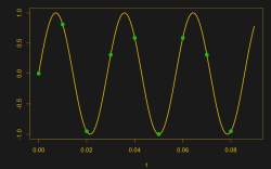
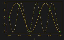
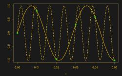
And then some spoil-sport comes along and draws in a version of your sine wave at -65 Hz, and then another at 135 Hz. And then more at -165 Hz and 235 Hz or -265 Hz and 335 Hz. And then an arbitrary number of potential sine waves that fit the very same data, all spaced apart at positive and negative integer multiples of your 100 Hz sampling frequency. Soon, your very pretty picture is looking a bit more complicated than you’d bargained for, and you have no idea which of these frequencies generated your data. It seems hopeless! You go home in tears.
But then you realize that this phenomenon gives you super powers — the power to resolve frequencies that are significantly higher than your sampling frequency. Just as the 235 Hz wave leaves an apparent 35 Hz waveform in the data when sampled at 100 Hz, a 237 Hz signal will look like 37 Hz. You can tell them apart even though they’re well beyond your ability to sample that fast. You’re pulling in information from beyond the Nyquist limit!
This essential ambiguity in sampling — that all frequencies offset by an integer multiple of the sampling frequency produce the same data — is called “aliasing”. And understanding aliasing is the first step toward really understanding sampling, and that’s the first step into the big wide world of digital signal processing.
Whether aliasing corrupts your pristine data or provides you with super powers hinges on your understanding of the effect, and maybe some judicious pre-sampling filtering, so let’s get some knowledge.
Aliasing

In some sense, aliasing is all in your mind. When you took your 100 Hz samples, you were probably looking for some relatively low frequency. Otherwise you would have sampled faster, right? But how is Mother Nature supposed to know which frequencies you want to measure? She just hands you the instantaneous sum of all voltage signals at all frequencies from DC to daylight, and leaves you to sort it out.
If you add together 35 Hz and 135 Hz waveforms, the resulting analog waveform will have twice the amplitude at the sampling points that correspond to 100 Hz. And when you sample, you get exactly the right value. Why did you expect otherwise?
The why is because when you think of the sampled values, you’re fooling yourself into thinking that you’ve seen the whole picture rather than just a few tiny points in time, with no data in between. But in principle, anything can be happening to the signal between samples. We just choose to use the simplest (lowest frequency) interpretation that will fit.
Not only does this seem reasonable, but this is also deeply ingrained in human physiology, so there’s no use fighting it. When you watch a Western, and the stagecoach accelerates so that the spokes in its wheels just match the film’s frame rate, you see the wheels as stopped because each frame was taken when the next spoke was in the same position as in the previous frame. As it speeds up further, you even think you see the wheel turning backwards. The illusion that sampled data comes from the “obvious” underlying signal is strong.
So if sampling adds together signals from different frequencies, how can we disentangle them? The short answer is that once the data has been collected, you can’t. There’s just not enough information there to recreate the full bandwidth of the universe.
But we can avoid aliasing when it’s a problem. The brute force method is to simply take more frequent samples. Since the alias frequencies are the desired frequency plus or minus integer multiples of the sampling frequency, 
Indeed, if you knew beforehand that your 35 Hz signal was contaminated with a 135 Hz signal, you could sample at 120 Hz, resulting in first-order aliases at -115 Hz and 15 Hz. Now you could separate the signals from each other using fancy DSP tricks. Of course, if the signal also has nuisance signals at 155 Hz, this won’t work.
Anti-Aliasing
An alternative is to get rid of the would-be aliases before sampling in the first place. When you wake up in the morning, and look outside to see the sun rise, you don’t ask yourself if you’ve slept for one night or two. That’s because it’s impossible that you’ve slept for 32 hours without noticing, right? Similarly, to anti-alias your data before sampling, you just need to rule out the higher multiples of the sampling frequency with a filter.
Lowpass sampling is the name for this procedure of applying a lowpass filter to your data before sampling it. Filtering out the high frequency content before sampling means that there’s nothing there to alias down, and the lowest frequencies, which you’re going to perceive as being “the sample” anyway, are the only ones present. This is done in nearly every analog-to-digital converter one way or another.
Because the negative frequencies interfere with our desired signal, the cutoff frequency of the filter needs to be set at 1/2 of the sampling frequency, or at the top of the desired bandwidth, whichever’s lower. When recording CDs, for instance, they are passed through a steep 20-22 Khz cutoff filter before being sampled at 44.1 kHz. A potentially contaminating 30.1 kHz signal, which would alias down to -14 kHz after sampling, is simply filtered away before it ever hits the ADC.
When you sample using an ADC, consider what’s going on at multiples of the sampling frequency. Do you need a lowpass filter? We suspect you might.
Bandpass Sampling
Finally, here is the super-power side of aliasing. Just as you can count the number of spokes on the “stopped” wagon wheel in Stagecoach, you can also get information about frequencies that are higher than the sampling rate by taking advantage of aliasing. And just as with the spokes on the wheel, even though it looks like you’re drawing samples from a single period of the waveform, you’re actually getting snapshots of different phase positions from across many periods of the wave. But if the desired signal is relatively consistent — the wagon’s spokes are roughly interchangeable — it won’t matter.
Bandpass Sampling (or undersampling) is the DSP name for this super power. You know that signals at all multiples of the sampling frequency are all going to get mixed together when you sample. The trick is just the same as in the lowpass case: simply filter out all the frequency bands except for the one that you want, and let aliasing do the frequency downconversion for you.
 So if we were interested in capturing the 135 Hz wave, we would simply filter as tightly around the desired 135 Hz as we can, sample at 100 Hz, and read the resulting frequency off at 35 Hz. Note that the ADC you use still has to be able to resolve the 135 Hz signal — if its input is too sluggish, it will smear out the high-frequency content, leaving you with a mess. (The exposure on the movie camera has to be fast enough to “freeze” the wagon wheel as well. Garbage in, garbage out.) Still, you can get the same information about the 135 Hz signal using only 100 samples per second instead of 270 by using this trick if your ADC is up to it.
More on Aliasing
There’s actually a lot more to aliasing than we have room to cover here, mostly because it informs all aspects of sampling, and thus DSP. If you want to get in deeper, any good DSP textbook should do. I really liked [Richard Lyons]’s “Understanding Digital Signal Processing”. (Here is the chapter on bandpass sampling for your enjoyment.)
If you’re a little bit uneasy with all of the “negative frequency” stuff above, it actually makes a lot more sense when viewed in the complex plane and with I/Q sampling. For a gentle video introduction to both complex signals and sampling theory, I like [Michael Ossmann]’s video series on software defined radio basics. Watch at least Chapter Six on complex numbers and then Chapter Nine on aliasing. If you don’t have any interest in SDR applications and you’re already comfortable with complex signals, you can actually get by starting Chapter Nine at 14:00 and going through 24:00. It’ll be the best ten minutes that you’ve spent. (Other than the ten reading this article, naturally.)
If you’re wondering just how those signals get sampled in the first place, try [Bil Herd]’s roundup of ADC techniques.


Thank you.
– someone who had to explain this a bit too often
I know I’m not the first – or even last – but I made a video on scope aliasing. https://www.youtube.com/watch?v=uWADu0aKk0w
Choosing the wrong ADC type for your application is just as problematic.
I thought Bil Herd covered this already. ;-)
Nah, a 741 voltage ramp comparator ought to be good enough for anyone. ;-)
This kind of aliasing is not a problem I’ve really thought about before, but I have an idea about that first example where you’re unable to tell the difference between a 35Hz sine wave from a 135Hz sine wave. What if you were to have independent hardware sampling the same signal at a different rate? I’d expect this process would generate different aliasing effects at each sample rate. Would these multiple sample rates allow you to derive the true frequency?
I imagine that you’d still have aliasing, but the aliasing frequencies would be based on the least common multiple of both sampling frequencies.
I boils down to amount of information, if you have more independent samples it is equivalent to a higher sample rate
why different rate? just shift phase of your two ADCs
thats what most oscilloscopes do internally nowadays – ADC interleaving. just make sure you have low jitter between them (I remember some rigol being really rubbish in this department until they fixed it with a patch changing clock driver settings).
Nice summary of 1940’s work which still applies for most purposes. However, David Donoho and Emmanuel Candes changed everything in 2004.
Aliasing is the result of periodic sampling in time using a comb function. The Fourier transform of which is also a comb. Multiplication in the time domain is convolution in the frequency domain. If the sampling is aperiodic in time, then the transform is a spike in frequency and there is no aliasing. A spike convolved with the input spectrum is the input spectrum. You still need “adequate” sampling, but that is actually about 1/5 of the traditional requirement.
It’s pretty mind boggling if you’ve spent 30 years following the gospel of Wiener-Shannon-Nyquist. But it’s true. There is a price to be paid in the form of a bunch of computation, but this is what underpins “compressive sampling” and things like the Rice single pixel camera.
The mathematics underlying this is the hairiest stuff I’ve ever done, but actually very simple to do in practice. If you want to get a better understanding of this, “A Wavelet Tour of Signal Processing” 3rd edition by Mallat will give you a good start. Donoho and Candes have lots of good papers on their websites, but they’re written at a very advanced level. “A Mathematical Introduction to Compressive Sensing” by Foucart and Rauhut was the first comprehensive treatment, but others have come out since. TI has implemented this in a spectrometer:
http://www.ti.com/tool/DLPNIRNANOEVM
They call it “Hadamard sampling” in their documentation.
Aperiodic sampling — very, very cool. Intuitively, it makes sense — if you sample at relatively prime time increments, it gets harder and harder (or higher and higher frequency) to fit an alias signal through.
Will have to do a quick read-up. Thanks!
Danger, Will Robinson!!!
Three years and several thousand pages later I’m still reading ;-)
The heart of the matter is solving Ax=y via L1 (least summed absolute error) instead of L2 (least squares). The FFT is an L2 solution on a Fourier basis. When I got involved in oil industry DSP in the early 80’s, all we could afford was L2 and barely that. We had a major crisis at work in ’82 when we started processing 120 channel, 2 ms, 3000 sample data and crushed an IBM mainframe with a vector processor until we split the datasets in pieces for that step (Wiener-Levinson predictive deconvolution).
What Donoho showed was that if a sparse L1 solution exists, then it is the unique solution to the L0 (optimal solution) problem which is NP-hard as it requires exhaustive search. The primary constraint is that the columns of A must have low correlation. We can now afford the computational cost of L1. This has lead to major advances in several areas:
compressive sensing (e.g. MRI data acquisition)
matrix completion (aka “The Netflix Problem)
identification of alleles related to genetic traits
the solution of ill-posed problems d = A*exp(a*t) + B*exp(b*t) (c.f. “Numerical Methods that Work”, p 253)
inverse problems and model selection (which of several competing equations best fit the data)
The list of things that were previously considered impossible grows by the day. IMHO the work of Candes and Donoho is the biggest thing in DSP since the 30’s and 40’s. Wavelet theory was closing in on it, but it took Candes and Donoho to make the conceptual leap.
This? https://en.wikipedia.org/wiki/Fast_Walsh%E2%80%93Hadamard_transform
Not really. I was a bit surprised that TI called it that.
Try these:
http://physicsbuzz.physicscentral.com/2006/10/single-pixel-camera.html
http://www.ece.rice.edu/~duarte/camera_news.html
google is unable to find a slew of papers it found previously. I’m not sure what the cause is.
Thanks, are they here, http://libgen.io/scimag/index.php?s=Single-Pixel%20Camera
The notion of being able to adequately sample a signal by using sparse sampling existed LONG before Donoho and Candes formalization made it fashionable. It’s been used in radio astronomy since the first arrays were used. Martin Gardiner popularized a form of it (the Golomb Ruler) in a Scientific American article in 1972. (RIP S.W. Golomb, last year). It’s been used in high precision laser spectroscopy since before 1986, when I first encountered it, and several other fields.
TANSTAAFL though: Do this at your noise floor’s peril. If you have a few bright spectral lines it works fine, but in the presence of noise or broadband signal or sampling jitter, it becomes crud. The formalism and the black art is figuring out what constitutes sufficient sampling to separate your desired signal from crud.
I’d not heard of Golomb’s work, but I agree that the idea has been around a long time. Donoho and Candes put it on a solid footing. It ONLY works if the signal has a sparse representation in some basis. If a 90% compressed version is acceptable, you can acquire the compressed version directly.
What they pointed out is that what matters is the information content rather than the apparent bandwidth. They don’t state it that way in anything I’ve read so far, but Shannon-Nyquist still applies.
This might be of interest:
http://www.edn.com/design/systems-design/4421064/Intuitive-sampling-theory–part-1
I’ve got around this problem by putting a random delay between samples. The randomization ensures there is only one reasonable frequency with a good fit. Didn’t even need a high performance ADC, the samples could be taken at more than 1 cycle.
Congratulations, you implemented sparse sampling! Basically, you sampled at the least common denominator sampling rate “lattice” that would contain all your sampling instants (if they’re truly random, let’s act as if there was a finite frequency that did that, and call the remainder “noise due to jitter), and then just omitted all the points in time not necessary to tell your signals apart :)
Stay away from that limit, give it 2 to 5 times the room and things are not so screwed up. First gen digital TV is a good example. 80’s CD’s another. Oversample.
Progress first and last, no turning back. The talk station in Indy on FM recently started using an inferior means of soda-strawing their studio to transmitting link that makes metallic tones that interleave thru what is normally heard as random noise in their signal. As in crowd noise in a game, now with little tones flirting in and out. Is this some of this sows ears junk retro sampling? Or did they just use a not for broadcast quality means of “upgrading” their link?
I have never heard this effect till now. I have heard it on some NPR links on an otherwise “working” station. However this station (WBAA) now is having fits of noise that are cyclic. This is on the BBC and the Met Opera, having lost a neighboring station (antenna problems-WVPE) I cannot compare signals live to know who is at fault.
A visual meme here is moire patterns showing up where none should be.
Isn’t the clever use of aliased information how structured illumination microscopy works?
https://en.wikipedia.org/wiki/Super-resolution_microscopy#Structured_illumination_microscopy_.28SIM.29
The way I understand it, the input illumination carries a modulation frequency (and orientation since it’s a 2D plane) which combines with the spatial pattern of the fluorophores in the sample. The illumination pattern is shifted in phase and orientation (I recall 9 samples per final image being necessary). The output is sampled at the Nyquist frequency for the ultimate resolution of the image, which is 2x higher than the optical transfer function of the system would normally allow.
Is this equivalent to saying the system (which can only sample up to a spatial frequency defined the optical transfer function) is sampling above that rate by having a biased signal applied that convolves with the unknown? Or, we measure the aliased response based on a convolution of a signal beyond our sampling rate with a known input signal?
This recent sample of XKCD seemed to fit the pattern.
https://xkcd.com/1814/
So, is this basically how those directional speakers that use ultrasound but you can hear normal range sound work?
Sort of… more like receiving a radio broadcast. A carrier signal is modulated with an audio signal. The result is the carrier with sum and difference frequencies that are well out of the audible range. As I understand it, this is normally done as a carrier and one sideband.
But when it hits a surface, the surface acts as a nonlinear device. This only works well when the sound pressure level is pretty high. Simplistically, the high pressure part of a sound wave has a pretty high limit, while the low pressure side can’t drop below a vacuum.
This causes the carrier to mix with the sidebands, causing sum and difference frequencies. The sum is even further out of the audible range, but the difference frequencies result in the original audio.
Works a bit like hanging up a wire and attaching a diode and earphones to it. The diode mixes the radio carrier with the sidebands, and the difference frequencies are the original audio.
For instance: 60kHz carrier, mix with a 2kHz tone. Result is a 60kHz carrier with a sideband at 62kHz. Feed this into directional ultrasonic speakers. This hits your head, mixes, and ignoring the sum frequencies, we get difference frequency of 2kHz.
As with a SSB AM radio transmission that does not suppress the carrier, the modulation should be at a max of 30% modulation to avoid distortion.
https://image.slidesharecdn.com/eeng3810chapter4-141012143102-conversion-gate02/95/eeng-3810-chapter-4-42-638.jpg
Thank you very very much!
Since I happen to be reading about Chebyshev and approximation: What if you replace the constant sample rate with a variable one? A VCXO that gets fed a signal with a period of 1 second?
From my reading of Chebyshev math, changing the period between samples should make it harder for high frequency signals to act as low frequency signals, because the required alias frequency keeps changing.
This is awsome!! i learnt it at college few days ago but you explain this easier, thanks man!