How Current Shunts Work

February 8, 2018 by Lewin Day 55 Comments

Current. Too little of it, and you can’t get where you’re going, too much and your hardware’s on fire. In many projects, it’s desirable to know just how much current is being drawn, and even more desirable to limit it to avoid catastrophic destruction. The humble current shunt is an excellent way to do just that.

Ohm’s Law.

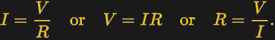
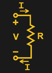
To understand current, it’s important to understand Ohm’s Law, which defines the relationship between current, voltage, and resistance. If we know two out of the three, we can calculate the unknown. This is the underlying principle behind the current shunt. A current flows through a resistor, and the voltage drop across the resistor is measured. If the resistance also is known, the current can be calculated with the equation I=V/R.

This simple fact can be used to great effect. As an example, consider a microcontroller used to control a DC motor with a transistor controlled by a PWM output. A known resistance is placed inline with the motor and, the voltage drop across it measured with the onboard analog-to-digital converter. With a few lines of code, it’s simple for the microcontroller to calculate the current flowing to the motor. Armed with this knowledge, code can be crafted to limit the motor current draw for such purposes as avoiding overheating the motor, or to protect the drive transistors from failure.

In fact, such strategies can be used in a wide variety of applications. In microcontroller projects you can measure as many currents as you have spare ADC channels and time. Whether you’re driving high power LEDs or trying to build protection into a power supply, current shunts are key to doing this.

Continue reading “How Current Shunts Work” →

Quantum Searching In Your Browser

February 7, 2018 by Al Williams 17 Comments

If you’ve made it through the last two posts on quantum computing (QC), then you’ve seen the Quirk simulator, a little of IBM’s web-based offering, and how entanglement and superposition can do strange and possibly wonderful things. However, the superdense encoding I showed you didn’t really feel like a real computer algorithm. This time we will look at Grover’s algorithm which is often incorrectly billed as an “unstructured database search.” In reality, it is an algorithm for making a state — that is a set of qubits — match some desired state without simply setting the state.

By analogy, consider a web service where you guess a number. Most discussions of Grover’s algorithm will tell you that the service will only tell you if the number is correct or not. If the number was from 1 to 16, using traditional computing, you’d have to query the values one at a time to see which is correct. You might get lucky and hit the first time. Or it might take 16 times. With qubits you can get the same result in only four attempts. In fact, if you try more times, you might get the wrong answer. Of course, what you really get is an answer that is probably correct, because that how QC works.

Continue reading “Quantum Searching In Your Browser” →

Quantum Weirdness In Your Browser

January 24, 2018 by Al Williams 29 Comments

I’ll be brutally honest. When I set out to write this post, I was going to talk about IBM’s Q Experience — the website where you can run real code on some older IBM quantum computing hardware. I am going to get to that — I promise — but that’s going to have to wait for another time. It turns out that quantum computing is mindbending and — to make matters worse — there are a lot of oversimplifications floating around that make it even harder to understand than it ought to be. Because the IBM system matches up with real hardware, it is has a lot more limitations than a simulator — think of programming a microcontroller with on debugging versus using a software emulator. You can zoom into any level of detail with the emulator but with the bare micro you can toggle a line, use a scope, and hope things don’t go too far wrong.

So before we get to the real quantum hardware, I am going to show you a simulator written by [Craig Gidney]. He wrote it and promptly got a job with Google, who took over the project. Sort of. Even if you don’t like working in a browser, [Craig’s] simulator is easy enough, you don’t need an account, and a bookmark will save your work.

It isn’t the only available simulator, but as [Craig] immodestly (but correctly) points out, his simulator is much better than IBM’s. Starting with the simulator avoids tripping on the hardware limitations. For example, IBM’s devices are not fully connected, like a CPU where only some registers can get to other registers. In addition, real devices have to deal with noise and the quantum states not lasting very long. If your algorithm is too slow, your program will collapse and invalidate your results. These aren’t issues on a simulator. You can find a list of other simulators, but I’m focusing on Quirk.

What Quantum Computing Is

As I mentioned, there is a lot of misinformation about quantum computing (QC) floating around. I think part of it revolves around the word computing. If you are old enough to remember analog computers, QC is much more like that. You build “circuits” to create results. There’s also a lot of difficult math — mostly linear algebra — that I’m going to try to avoid as much as possible. However, if you can dig into the math, it is worth your time to do so. However, just like you can design a resonant circuit without solving differential equations about inductors, I think you can do QC without some of the bigger math by just using results. We’ll see how well that holds up in practice.

Continue reading “Quantum Weirdness In Your Browser” →

Skin (Effect) In The Game

November 22, 2017 by Al Williams 70 Comments

We love to pretend like our components are perfect. Resistors don’t have capacitance or inductance. Wires conduct electricity perfectly. The reality, though, is far from this. It is easy to realize that wire will have some small resistance. For the kind of wire lengths you usually encounter, ignoring it is acceptable. If you start running lots of wire or you are carrying a lot of current, you might need to worry about it. Really long wires also take some time to get a signal from one end to the other, but you have to have a very long wire to really worry about that. However, all wires behave strangely as frequency goes up.

Of course there’s the issue of the wire becoming a significant part of the signal’s wavelength and there’s always parasitic capacitance and inductance. But the odd effect I’m thinking of is the so-called skin effect, first described by [Horace Lamb] in 1883. [Lamb] was working with spherical conductors, but [Oliver Heaviside] generalized it in 1885.

Put simply, when a wire is carrying AC, the current will tend to avoid traveling in the center of the wire. At low frequencies, the effect is minimal, but as the frequency rises, the area in the center that isn’t carrying current gets larger. At 60 Hz, for example, the skin depth for copper wire — the depth where the current falls below 1/e of the value near the surface — is about 0.33 inches. Wire you are likely to use at that frequency has a diameter less than that, so the effect is minimal.

However, consider a 20 kHz signal — a little high for audio unless you are a kid with good ears. The depth becomes about 0.018 inches. So wire bigger than 0.036 inches in diameter will start losing effective wire size. For a 12-gauge wire with a diameter of 0.093 inches, that means about 25% of the current-handling capacity is lost. When you get to RF and microwave frequencies, only the thinnest skin is carrying significant current. At 6 MHz, for example, copper wire has a skin depth of about 0.001 inches. At 1 GHz, you are down to about 0.000081 inches. You can see this (not to scale) in the accompanying image. At DC, all three zones of the wire carry current. At a higher frequency, only the outer two zones carry significant current. At higher frequencies, only the outer zone is really carrying electrons.

Continue reading “Skin (Effect) In The Game” →

Switching: From Relays To Bipolar Junction Transistors

September 7, 2017 by Sean Boyce 28 Comments

How many remote controls do you have in your home? Don’t you wish all these things were better integrated somehow, or that you could add remote control functionality to a random device? It’s a common starting point for a project, and a good learning experience for beginners.

A common solution we’ve seen applied is to connect a relay in parallel to all the buttons we want to press. When the relay is triggered, for example by your choice of microcontroller, it gets treated as a button press. While it does work, relays are not really the ideal solution for the very low current loads that we’re dealing with in these situations.

As it turns out, there are a few simple ways to solve this problem. In this article, we’re going to focus on using common bipolar junction transistors instead of relays to replace physical switches. In short, how to add transistors to existing electronics to control them in new ways.

Continue reading “Switching: From Relays To Bipolar Junction Transistors” →

Designing For Fab: A Heads-Up Before Designing PCBs For Professional Assembly

May 10, 2017 by Sonya Vasquez 55 Comments

Designing pcbs for assembly is easy, right? We just squirt all the footprints onto a board layout, connect all the traces, send out the gerbers and position files, and we’re done–right?

Whoa, hold the phone, there, young rogue! Just like we can hack together some working source code with variables named after our best friends, we can also design our PCBs in ways that make it fairly difficult to assemble.

However, by following the agreed-upon design specs, we’ll put ourselves on track for success with automated assembly. If we want another party to put components on our boards, we need to clearly communicate the needed steps to get there. The best way to do so is by following the standards.

Proper Footprint Orientation

Now, for a moment, let’s imagine ourselves as the tip of a vacuum pickup tool on a pick-and-place machine. These tools are designed to pick up components on the reel from their centroid and plunk them on their corresponding land pattern. Seems pretty straightforward, right? It is, provided that we design our footprints knowing that they’ll one day come face-to-face with the pick-and-place machine.

To get from the reel to the board, we, the designers, need two bits of information from out part’s datasheet: the part centroid and the reel orientation.

The part centroid is an X-Y location that calls out the center-of-mass of the part. It basically tells the machine: “pick me up from here!” As designers, it’s our responsibility to design all of our footprints such that the footprint origin is set at the part’s centroid. If we forget to do so, the pick-and-place will try to suck up our parts from a location that may not stick very well to the package, such as: the corner.

Continue reading “Designing For Fab: A Heads-Up Before Designing PCBs For Professional Assembly” →

Say It With Me: Aliasing

March 23, 2017 by Elliot Williams 28 Comments

Suppose you take a few measurements of a time-varying signal. Let’s say for concreteness that you have a microcontroller that reads some voltage 100 times per second. Collecting a bunch of data points together, you plot them out — this must surely have come from a sine wave at 35 Hz, you say. Just connect up the dots with a sine wave! It’s as plain as the nose on your face.

And then some spoil-sport comes along and draws in a version of your sine wave at -65 Hz, and then another at 135 Hz. And then more at -165 Hz and 235 Hz or -265 Hz and 335 Hz. And then an arbitrary number of potential sine waves that fit the very same data, all spaced apart at positive and negative integer multiples of your 100 Hz sampling frequency. Soon, your very pretty picture is looking a bit more complicated than you’d bargained for, and you have no idea which of these frequencies generated your data. It seems hopeless! You go home in tears.

But then you realize that this phenomenon gives you super powers — the power to resolve frequencies that are significantly higher than your sampling frequency. Just as the 235 Hz wave leaves an apparent 35 Hz waveform in the data when sampled at 100 Hz, a 237 Hz signal will look like 37 Hz. You can tell them apart even though they’re well beyond your ability to sample that fast. You’re pulling in information from beyond the Nyquist limit!

This essential ambiguity in sampling — that all frequencies offset by an integer multiple of the sampling frequency produce the same data — is called “aliasing”. And understanding aliasing is the first step toward really understanding sampling, and that’s the first step into the big wide world of digital signal processing.

Whether aliasing corrupts your pristine data or provides you with super powers hinges on your understanding of the effect, and maybe some judicious pre-sampling filtering, so let’s get some knowledge.

Continue reading “Say It With Me: Aliasing” →