Say It With Me: Root-Mean-Square

April 13, 2017 by Elliot Williams 23 Comments

If you measure a DC voltage, and want to get some idea of how “big” it is over time, it’s pretty easy: just take a number of measurements and take the average. If you’re interested in the average power over the same timeframe, it’s likely to be pretty close (though not identical) to the same answer you’d get if you calculated the power using the average voltage instead of calculating instantaneous power and averaging. DC voltages don’t move around that much.

Try the same trick with an AC voltage, and you get zero, or something nearby. Why? With an AC waveform, the positive voltage excursions cancel out the negative ones. You’d get the same result if the flip were switched off. Clearly, a simple average isn’t capturing what we think of as “size” in an AC waveform; we need a new concept of “size”. Enter root-mean-square (RMS) voltage.

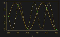
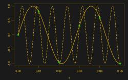
To calculate the RMS voltage, you take a number of voltage readings, square them, add them all together, and then divide by the number of entries in the average before taking the square root: $\sqrt{\frac{1}{n} \left(v_1^2 + v_2^2 +...+ v_n^2\right)}$ . The rationale behind this strange averaging procedure is that the resulting number can be used in calculating average power for AC waveforms through simple multiplication as you would for DC voltages. If that answer isn’t entirely satisfying to you, read on. Hopefully we’ll help it make a little more sense.

Continue reading “Say It With Me: Root-Mean-Square” →

Say It With Me: Aliasing

March 23, 2017 by Elliot Williams 28 Comments

Suppose you take a few measurements of a time-varying signal. Let’s say for concreteness that you have a microcontroller that reads some voltage 100 times per second. Collecting a bunch of data points together, you plot them out — this must surely have come from a sine wave at 35 Hz, you say. Just connect up the dots with a sine wave! It’s as plain as the nose on your face.

And then some spoil-sport comes along and draws in a version of your sine wave at -65 Hz, and then another at 135 Hz. And then more at -165 Hz and 235 Hz or -265 Hz and 335 Hz. And then an arbitrary number of potential sine waves that fit the very same data, all spaced apart at positive and negative integer multiples of your 100 Hz sampling frequency. Soon, your very pretty picture is looking a bit more complicated than you’d bargained for, and you have no idea which of these frequencies generated your data. It seems hopeless! You go home in tears.

But then you realize that this phenomenon gives you super powers — the power to resolve frequencies that are significantly higher than your sampling frequency. Just as the 235 Hz wave leaves an apparent 35 Hz waveform in the data when sampled at 100 Hz, a 237 Hz signal will look like 37 Hz. You can tell them apart even though they’re well beyond your ability to sample that fast. You’re pulling in information from beyond the Nyquist limit!

This essential ambiguity in sampling — that all frequencies offset by an integer multiple of the sampling frequency produce the same data — is called “aliasing”. And understanding aliasing is the first step toward really understanding sampling, and that’s the first step into the big wide world of digital signal processing.

Whether aliasing corrupts your pristine data or provides you with super powers hinges on your understanding of the effect, and maybe some judicious pre-sampling filtering, so let’s get some knowledge.

Continue reading “Say It With Me: Aliasing” →

Say It With Me: Input Impedance

July 29, 2015 by Elliot Williams 37 Comments

In the “Say It with Me” series, we’ll take a commonly used concept out of electronics and explain it the best we can. If there’s something that’s been bugging you, or a certain term or concept that keeps cropping up in your projects, let us know. We’ll write about it!

What’s up with input impedance? You hear people talking about it, but why does it matter? And impedance matching? Let’s break it all down.

First of all, impedance is the frequency-dependent sister of resistance, so for intuition we’ll first work through the cases of purely resistive impedance. And that’s almost fine if you’re only ever working at one frequency. We’ll hint at the full-blown impedance = resistance + reactance version at the end, but it’s really its own topic. For now, pretend that your circuits aren’t reactive.

Continue reading “Say It With Me: Input Impedance” →