[Michael Ossmann] spoke on Friday to a packed house in the wireless hacking village at DEF CON 25. There’s still a day and a half of talks remaining but it will be hard for anything to unseat his Reverse Engineering Direct Sequence Spread Spectrum (DSSS) talk as my favorite of the con.
DSSS is a technique used to transmit reliable data where low signal strength and high noise are likely. It’s used in GPS communications where the signal received from a satellite is often far too small for you to detect visually on a waterfall display. Yet we know that data is being received and decoded by every cell phone on the planet. It is also used for WiFi management packets, ZigBee, and found in proprietary systems especially any dealing with satellite communications.
[Michael] really pulled a rabbit out of a hat with his demos which detected the DSSS signal parameters in what appeared to be nothing but noise. You can see below the signal with and without noise; the latter is completely indiscernible as a signal at all to the eye, but can be detected using his techniques.


Detecting DSSS with Simple Math
 [Michael] mentioned simple math tricks, and he wasn’t kidding. It’s easy to assume that someone as experienced in RF as he would have a different definition of ‘simple’ than we would. But truly, he’s using multiplication and subtraction to do an awful lot.
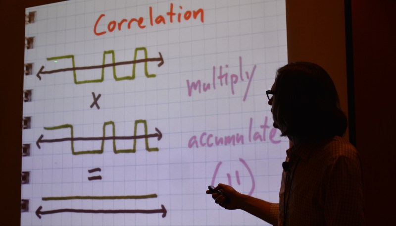
DSSS transmits binary values as a set called a chip. The chip for digital 1 might be 11100010010 with the digital 0 being the inverse of that. You can see this in the slide at the top of this article. Normal DSSS decoding compares the signal to expected values, using a correlation algorithm that multiplies the two and gives a score. If the score is high enough, 11 in this example, then a bit has been detected.
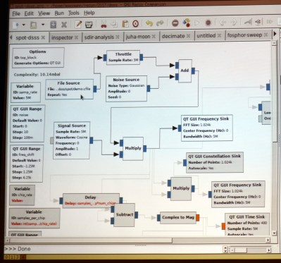
To reverse engineer this it is necessary to center on the correct frequency and then detect the chip encoding. GNU radio is the tool of choice for processing a DSSS capture from a SPOT Connect module designed to push simple messages to a satellite communication network. The first math trick is to multiply the signal by itself and then look at spectrum analysis to see if there is a noticeable spike indicating the center of the frequency. This can then be adjusted with an offset and smaller spikes on either side will be observed.
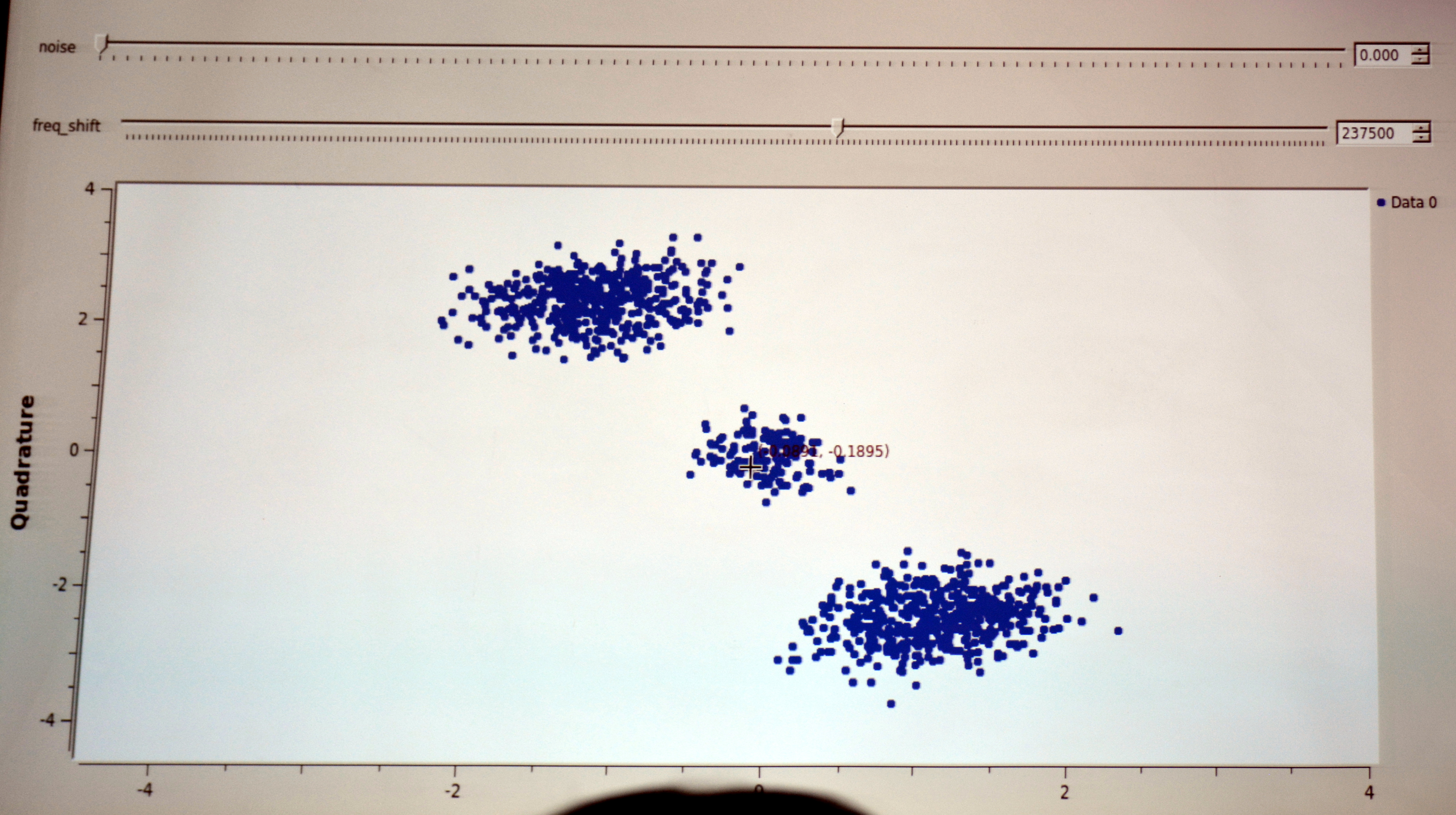 When visualized in a constellation view you begin to observe a center and two opposite clusters. The next math trick is to square the signal (multiply it by itself) and it will join those opposite clusters onto one side. What this accomplishes is a strong periodic component (the cycle from the center to the cluster and back again) which reveals the chip rate.
Detecting symbols within the chip is another math trick. Subtract each successive value in the signal from the last and you will mostly end up with zero (high signal minus high signal is zero, etc). But every time the signal spikes you’re looking at a transition point and the visualization begins to look like logic traced out on an oscilloscope. This technique can deal with small amounts of noise but becomes more robust with a bit of filtering.

This sort of exploration of the signal is both fun and interesting. But if you want to actually get some work done you need a tool. [Michael] built his own in the form of a python script that cobbles up a .cfile and spits out the frequency offset, chip rate, chip sequence length, and decoded chip sequence.
Running his sample file through with increasing levels of noise added, the script was rock solid on detecting the parameters of the signal. Interestingly, it is even measuring the 3 parts per million difference between the transmitter and receiver clocks in the detected chip rate value. What isn’t rock solid is the actual bit information, which begins to degrade as the noise is increased. But just establishing the parameters of the protocol being used is the biggest part of the battle and this is a dependable solution for doing that quickly and automatically.
You can give the script a try. It is part of [Michael’s] Clock Recovery repo. This talk was recorded and you should add it to your reminder list for after the con when talks begin to be published. To hold you over until then, we suggest you take a look at his RF Design workshop from the 2015 Hackaday Superconference.


DSSS is the kind of story I like to see on Hackaday.
Wow.
This is amazing. Why do I feel the same way I felt in my
Schoolboy neurotic dreams when I dreamt of sitting in my math class without any clothes.
This potentially exposes a lot of information.
“The first math trick is to multiply the signal by itself” > This is known as auto-correlation. The sequences used in DSSS have good auto-correlation properties. This is why complimentary codes are used for this.
https://en.wikipedia.org/wiki/Barker_code
https://en.wikipedia.org/wiki/Complementary_code_keying
Also https://en.wikipedia.org/wiki/Gold_code
https://www.youtube.com/watch?v=wyEKakfqNkk
That would be “complementary” codes.
Does anyone know if talks like these from DEF CON are published?
they usually post slides with the video later on.
They will be uploaded to their youtube channel a month or two after the convention.
https://www.youtube.com/user/DEFCONConference/videos
It used to be 9+ months, has this been improved
Thanks for visiting us to Wireless Village Mike! Come visit us again.
Mark
Wireless Village
I met Michael as his HackRF stand at HITB a couple years back, sound guy, He took interest in my own OSHW project and we traded kicad tips. Cool to see he’s killing it in the RF hacking field still. can’t wait to watch the video when DEFCON put it out.
SD.
I love the concert.
My solution would be to have a dynamic chip that changes for every single bit being broadcast. So instead of “1” being a static 11100010010 and “0” being a static 00011101101 use a 64 bit maximal length LFSR feedback polynomial and invert the bits if it is a zero being transmitted. It does mean that the location within the Linear-feedback shift register needs to be know to both the transmitter and receiver and their clocks need to be kept perfectly in sync. If there is a slightly drift in synchronization, provided there is enough processing power and RAM to store some historical and future codes in memory, at the receiver, it can re-sync from the transmitter.
The the problem is then one of identifying a LFSR, which could be run through a hashing function to make it look even more like random noise.
You could do away with the LFSR and use a shared key encrypted bit stream.
This is done in practice. See the GPS p(y) signal
” But truly, he’s using multiplication and subtraction to do an awful lot.”
Handy when one doesn’t have a high-powered chip doing the work.
Since correlation in time is multiplication in frequency, you can take the FFTs of both the RX signal, and PN code, then multiply. The correlation peak is then at the PN code offset.
What is DSSS and why is hacking it fascinating?
I want to slurp in some new knowledge.
Please help me digest!
I’ve heard about hiding in the noise floor in respects to transmitting data, Never knew it would only require simple maths to recover.
A method of noise floor transmission and recovery like this added to a newer gen of WiFi or BTLE, I’d guess would help with power saving and/or useful for a slower transmitting speed when the portable PC goes just out of range of the transmitter.
US military has been using DSSS for a long time, they classify DSSS radios as LPI (Low Probability of Intercept) and LPD (Lower Probability of Detection)
AN/PRC-343 is a good example of a DSSS radio. Cheap, super simple, low range, long talk time, reliable.
uh, I forgot the teardown pr0n http://www.milspec.ca/radspec/prc-343.html
just look how clean and simple it is inside
http://www.milspec.ca/radspec/images/prc-343/PRC-343_digital_in_open_case.jpg
now if we can just write some appropriate code to run on last year’s bitcoin mining ASIC modules, we’ll be in business…
Hello! Very nice information!! However, can I ask one question about this part :”The first math trick is to multiply the signal by itself and then look at spectrum analysis to see if there is a noticeable spike indicating the center of the frequency. This can then be adjusted with an offset and smaller spikes on either side will be observed.”
The question is — multiplying the incoming signal with itself will mean squaring the signal. So if the incoming signal is like:
d(t).p(t).cos(wt) + d(t).p(t).sin(wt) …. then squaring it would give something like:
(d.p)^2.cos^2(wt) + (d.p)^2.sin^2(wt) + 2.(d.p)^2.cos(wt).sin(wt), where the (d.p)^2 becomes a constant value. We could arbitrarily treat it (d.p)^2 as 1 if normalised. So we’d end up with:
cos^2(wt) + sin^2(wt) + 2.cos(wt).sin(wt), where the first two terms cos^2 + sin^2 is mathematically equal to 1.
So the above becomes: 2.cos(wt).sin(wt). So this means we don’t expect to see any spikes associated with the pseudorandom sequence code rate when we square the incoming signal, right?
Thanks!
oops… for the last equation, I should have typed: 1 + 2.cos(wt).sin(wt). I also omitted phase shift ‘phi’ in the incoming signal for simplicity.