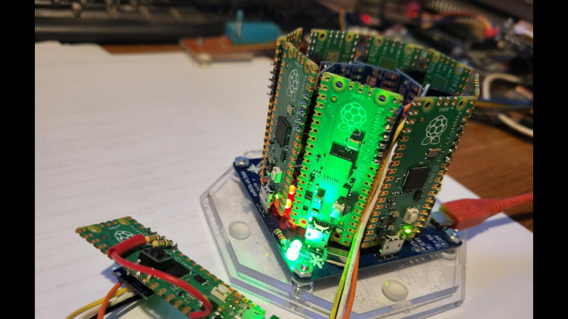
[ExtremeElectronics] cleverly demonstrates that if one Raspberry Pi Pico is good, then nine must be awesome. The PicoCray project connects multiple Raspberry Pi Pico microcontroller modules into a parallel architecture leveraging an I2C bus to communicate between nodes.
The same PicoCray code runs on all nodes, but a grounded pin on one of the Pico modules indicates that it is to operate as the controller node. All of the remaining nodes operate as processor nodes. Each processor node implements a random back-off technique to request an address from the controller on the shared bus. After waiting a random amount of time, a processor will check if the bus is being used. If the bus is in use, the processor will go back to waiting. If the bus is not in use, the processor can request an address from the controller.
Once a processor node has an address, it can be sent tasks from the controller node. In the example application, these tasks involve computing elements of the Mandelbrot Set. The particular elements to be computed in a given task are allocated by the controller node which then later collects the results from each processor node and aggregates the results for display.
The name for this project is inspired by Seymore Cray. Our Father of the Supercomputer biography tells his story including why the Cray-1 Supercomputer was referred to as “the world’s most expensive loveseat.” For even more Cray-1 inspiration, check out this Raspberry Pi Zero Cluster.


I’m curious – is this actually useful for something, or is it a “because I can” project? That MCU is very versatile, but I wonder if there’s any scenario where this setup is more practical for parallel computing than a multicore CPU.
This is just for fun, I would assume, given that the nodes are weak and connected through a slow I2C bus.
I suppose they could be connected via the USB bus as well to improve speed, but that probably would imply developing a specific USB layer.
there is enough gpio to set up an 8-bit ring bus or a 16-bit shared bus, and that could operate as fast if not faster than i2c. you have to roll your own protocol but that’s all part of the fun.
Especially fast with the programmable IO.
I guess this one is just for fun. Some low-performance clusters are used for educational/research purposes, though (probably not this one, because and just because it won’t run existing software/libraries).
As said on github:
“This code is only a proof of concept. For many uses, it actually runs slower than running on a single pico. ”
The PIO could probably be used for a faster interface
+1 wud have loved to see it utilizing PIO
Looks like using a RPi as a Transputer.
Transputer. That is a term I have not heard since…
If you only knew the power of the…
Occam programming language.
People figured out that coherent shared memory is the best way to parallelize multiple processors. Only when that’s no longer an option do you go for network connected nodes.
Nice, but where’s the liquid nitrogen, and the parakeet sized loveseat? Seriously, nice job.
It used Fluorinert liquid for cooling, not nitrogen.
The Cray 1 used Freon (probably R-12) which dumped its heat into a fountain in the case of the software development HQ. You could spot that building when flying into MSP in winter by the huge steam cloud coming off the fountain. Other locations used traditional cooling stacks. The Cray 2 used 3M Fluorinert.
where is `tight_loop_contents();` defined?
It reminds me of [Steve Ciarcia]’s cluster computer using 8051 cards controlled by an IBM PC. That, too, was used to generate Mandelbrot sets. The articles were serialized in Byte Nov ’88 to Jan ’89.
It’s hard enough to find 1 raspberry pi. Now you need 9 to build this thing.
These are picos though, they aren’t that difficult to get AFAIK.
Same thing 7 years ago see https://hackaday.com/2016/12/19/80-pic32-cluster-does-fractals/
The compiler support on PIC32 is so dreadful, might as well not exist. File under “who cares”
His name was Seymour, not Seymore.
Mr Butts?
I wonder what kind of throughput they could get if attached via DMA’d PIO…
In 1985, I did a similar project for the EPA while at the Research Triangle Institute in NC. The EPA had an atmospheric chemistry model covering the NE US with a 42 X 60 X 3 grid (7560 locations). The model was a set of partial differential equations (PDEs) and computed the changes in 23 atmospheric constituents due to interactions between them and energy gains from isolation and loses due to radiation. These played against recorded weather data that governed the simulated air mass movement. The basic scenario was to compute the changes for the air mass that started at each at each grid point for a 30 minute interval, compute its location at the end of the interval and interpolate back to the grid points. Some 90% of the computation went to solving the PDEs and 10% to doing the interpolations. While this looks like a parallel computing problem at first glance, running the code on the CRAYs of the day gave relatively little speedup because the stiffness of the PDEs was a strong function of the concentrations of some of the constituents and the PDE solver used adaptive step sizes to speed up the process. Most of the cells could be solved quickly using larger integration step sizes but a few were very slow. Parallel solutions imposed the minimum step size on all cells. This is a characteristic of a multiple instruction stream, multiple data stream problem. Computing a single cell on a VAX 750 took about 300 bytes of input and took between a few seconds and several minutes to produce a similar amount of output.
Our solution was a bunch of microVAX workers on an ethernet with a larger VAX acting as the controller / dispatcher. It also did the interpolations. At the start of each cycle, cell data was sent to each of the workers. As a worker reported back, it was given another cell. Cells were dispatched so that the cells that had taken the longest compute times in the previous round were dispatched early, while the fast cells were saved until last. The nature of the chemistry and physics involved resulted in relatively small changes between rounds, so this was very effective.
The whole project was fraught with politics – the EPA computer center director had hoped to use the model to justify a real supercomputer, but the machine we designed was built and used successfully for some period.
I2C wouldn’t be my first choice. It’s too slow and can crash easily with many implementations.
As a point of interest, yhe circuit boards in a Cray supercomputer were mounted so that they radiated out from the central column. Not forming the sides of an octagon as these boards are.
This was to keep the length of the common bus to a minimum and still allow the cooling equipment to be fitted between the boards.