A while back, I posted a review of the Analog Discovery 2, which is one of those USB “do everything” instruments. You might recall I generally liked it, although I wasn’t crazy about the price and the fact that the BNC connectors were an extra item. However, in that same post, I mentioned I’d look at the device’s capabilities as a network analyzer (NA) sometime in the future. The future, as they say, is now.

What’s an NA?

In its simplest form, there’s not much to an NA. You sweep a frequency generator across some range of frequencies. You feed that into some component or network of components and then you measure the power you get out compared to the power you put in. Fancy instruments can do some other measurements, but that’s really the heart of it.

The output is usually in two parts. You see a scope-like graph that has the frequency as the X-axis and some sort of magnitude as the Y-axis. Often the magnitude will be the ratio of the output power to the input power as a decibel. In addition, another scope-like output will show the phase shift through the network (Y-axis) vs frequency (X-axis). The Discovery 2 has these outputs and you can add custom displays, too.

Why do you care? An NA can help you understand tuned circuits, antennas, or anything else that has a frequency response, even an active filter or the feedback network of an oscillator. Could you do the same measurements manually? Of course you could. But taking hundreds of measurements per octave would be tedious and error-prone.

Set Up

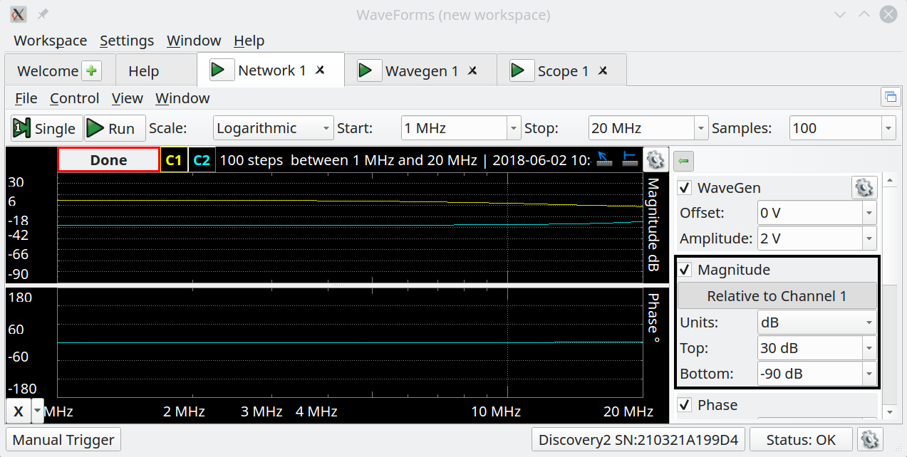
The software setup is easy and works like all the other functions on the Discovery 2. You create a “network” instrument and the most common settings you’ll want to adjust are along the top. You can select a linear or log scale on the X-axis. You also can pick the minimum and maximum sweep frequency, along with the number of samples to take. Along the right, you can select the voltage output of the wave generator, if you care. You can also set the Y-axis units along with the gain on the channels.

The device works by connecting the scope’s channel 1 probe to the input of the device under test and then connecting channel 2 to the output. The input of the device also connects to the wave generator output and you will want to make sure all the grounds are wired together, too. You can see the Digilent video on how to use this mode of the device at the end of this post.

Start Simple

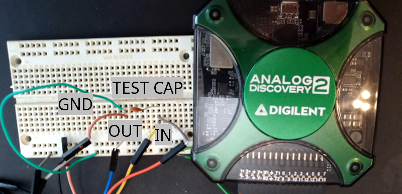
The simplest interesting thing you could look at would be a capacitor. However, this shows a few of the flaws of the Discovery 2. The way the flying leads are set up, it is pretty hard to make good connections for something like this. The BNC accessory would be a little easier. At least it would allow for more types of test leads to easily attach. I elected to put some wires into the flying leads and connect the wires to a breadboard.

The obvious problem with that is the breadboard has its own capacitance along with some crosstalk. With an open circuit, you ought to get a flat line of 0 dB for the reference signal (green in the screenshot above) and more or less negative infinity on the blue trace which is the signal through the test network. As you can see, however, the signal starts to curve around 3 MHz and really has problems at 10 MHz. I do not think this is inherent in the instrument, but a byproduct of the poor test leads and the effects of the solderless breadboard.

Here’s a 10 pF capacitor’s curve:

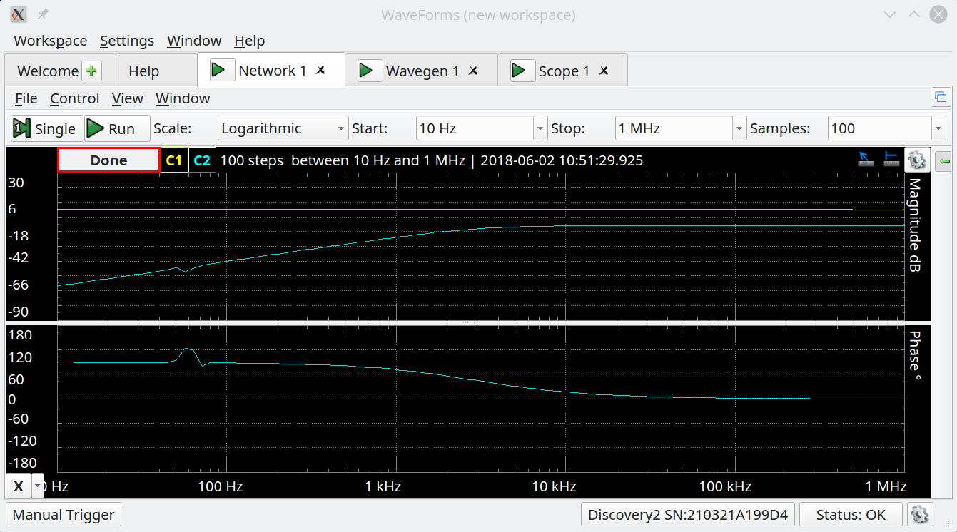
I assume the little bump at 60 Hz is an artifact of noise from the AC power line either conducted through the USB cable or picked up from the air. The device comes with a USB cable that has an integrated ferrite core but I used whatever happened to be hanging off my computer, so that may explain that.

You can see the response is what you’d expect from a capacitor. High loss at low frequencies, getting better until it levels off at some higher frequency. Note the left side of the graph is at 10 Hz. The instrument is noticeably slow making readings at that frequency. It appears it waits for a certain number of cycles, not a certain period of time, so the reading gets faster as the sweep frequency increases. If you accidentally enter mHz instead of MHz into of the boxes, you will get millihertz and very long runtimes indeed. An important lesson.

Resonant

Next, I put a 100 uH inductor in place of the capacitor. This doesn’t look like you would expect unless you realize that the inductor is going to resonate with the parasitic capacitance from the breadboard and the leads. Here’s the plot:

The peak is about 2.5 MHz so you can calculate that the test setup has just under 41 pF of stray capacitance. That ignores the effect of stray inductance, but with this setup, I think it is fair to assume that will be relatively small at these frequencies. From the shape of the peak, the capacitance is mostly in series because the signal is making it through. Good to know. However, if you ignore the peak, you can see the expected inductor behavior of dropping as frequency increases.

By the way, pumping a volt through the inductor at resonance causes a large spike which messes up the plot. The instrument protects itself and shows a message that it is out of range. The answer is to turn down the wave’s output voltage on the right-hand panel.

I next put 20 pF across the inductor. In theory, this should resonate at about 3.56 MHz. That doesn’t account for the extra capacitance or the tolerance of the components, for that matter.  The real figure worked out to about 3.4 MHz, as you can see below.

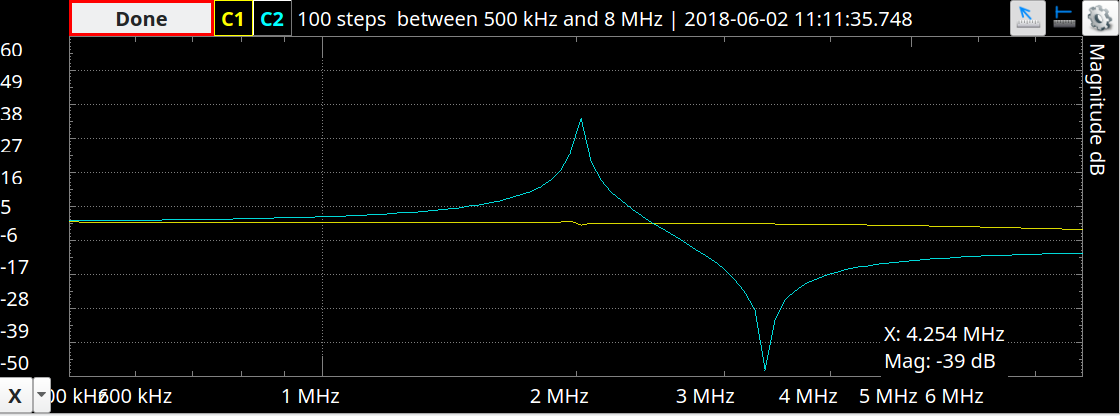
Note, you can still see the spurious series spike, but it has also changed frequency due to the additional capacitance introduced.

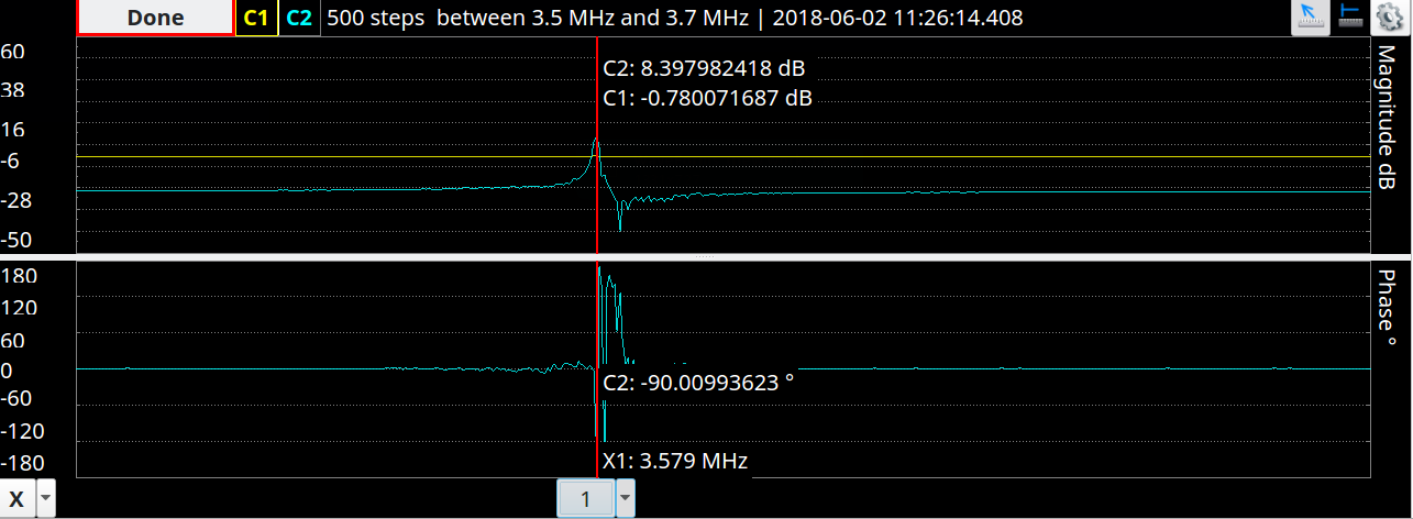
Crystal Method

For fun, I took all the other components out and grabbed a colorburst crystal from an old-style TV.  You can see from the figure below that the series peak is right on the money for frequency. Notice the frequency is close, but different, where it is in parallel resonance. That’s why when you specify a crystal, you have to call out if you are looking for the series or parallel resonant frequency.

Just for Fun

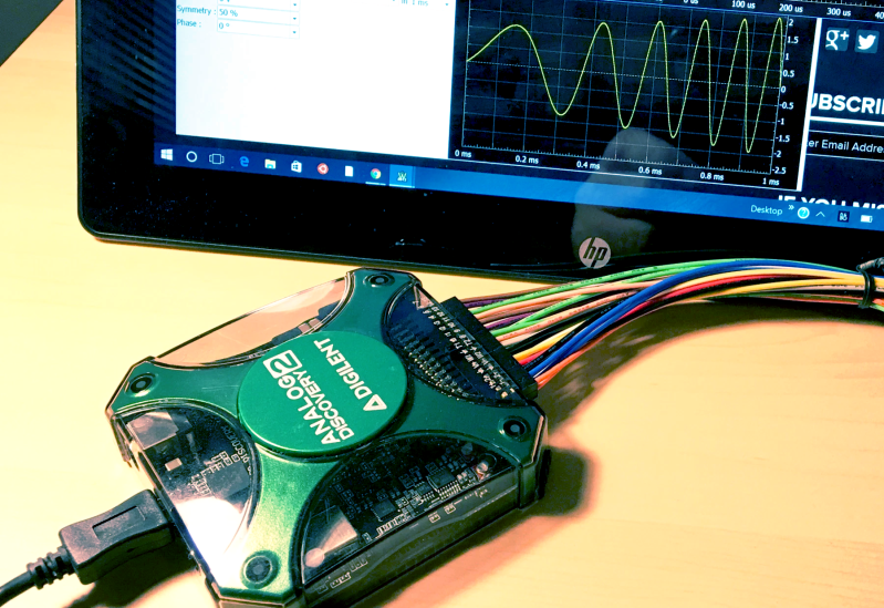
Because the NA is such a simple layout and since the NA uses the scope and waveform leads, I thought it would be interesting to manually set the frequency generator and look at the scope without relying on the NA instrument itself. You can see in the video below that it is satisfying to watch the response change with frequency.  I set the sweep to take five seconds to make it easier to watch.

Notice that the blue FFT spike gets bigger as it moves toward resonance. You can also see the scope trace get bigger. Note that the blue oscilloscope trace is on a more sensitive scale than the yellow source trace. They are not close to the same magnitude despite appearances. Also remember that voltage on the scope doesn’t translate directly into power. A 5 V signal at 1 A has more power than a 10 V signal at 10 mA.

Conclusion

I only looked at a few passive examples, but you could use this device to measure antennas, active filters, or anything with a frequency response. Just be careful with grounds and not to put out too much signal for the device under test. You may have noticed that while you get magnitude and phase information, you don’t get some measurements you’d expect on a very pricey instrument made just for this purpose (like VSWR).

Is the Discover 2’s NA mode useful? Yes. Is it perfect? No. The interconnect issue gets more and more problematic the higher you go in frequency. If you already have one of these, by all means, use the NA, especially for lower frequency work. But if you really need an NA, this probably isn’t going to be your first choice.

There are network analyzers out there that are affordable although they may have odd frequency ranges. For example, we recently saw one for $150 that won’t go below 137 MHz. It will, however, go up to 2.4 GHz. If you want more background, we had an article on this whole class of devices before. You might also enjoy Digilent’s video on how to set up the network analyzer, below.