
Bandwidth is one of those technical terms that has been overloaded in popular speech: as an example, an editor might ask if you have the bandwidth to write a Hackaday piece about bandwidth. Besides this colloquial usage, there are several very specific meanings in an engineering context. We might speak about the bandwidth of a signal like the human voice, or of a system like a filter or an oscilloscope — or, we might consider the bandwidth of our internet connection. But, while the latter example might seem fundamentally different from the others, there’s actually a very deep and interesting connection that we’ll uncover before we’re done.
Let’s have a look at what we mean by the term bandwidth in various contexts.
Digital Bandwidth
 Perhaps the most common usage of the term bandwidth is for the data bandwidth of digital channels, in other words, the rate of information transfer. In this case, it’s measured in bits per second. Your ISP might provision you 50/10 Mbps internet service for example, meaning you have 50 million bits per second of download capacity and 10 million bits per second of upload. In this case you would say that the download bandwidth is 50 Mbps. Measuring the digital bandwidth of a network channel is as easy as sending a fixed number of bits and timing how long it takes; this is what those broadband speed test sites do.
We’ll come back to digital bandwidth in a little while, to see how it’s connected to the next concept, that of signal bandwidth.
Signal Bandwidth
 The term bandwidth is also used to describe the frequency range occupied by a signal. In this case, the bandwidth of the signal is defined as the maximum frequency contained in the signal minus the minimum frequency. If a signal has frequency components between 100 Hz and 300 Hz, we would say that the signal has a bandwidth of 200 Hz. As a concrete example, consider the medium-wave (aka AM) broadcast band in the US: each signal occupies a bandwidth of 20.4 kHz. So, a transmitter operating on the 1000 kHz channel should only output frequencies between 989.8 kHz and 1010.2 kHz. It’s interesting to note that an AM-modulated RF signal takes up twice the bandwidth of the transmitted audio, since both frequency sidebands are present; that 20.4 kHz RF bandwidth is being used to send audio with a maximum bandwidth of 10.2 kHz.
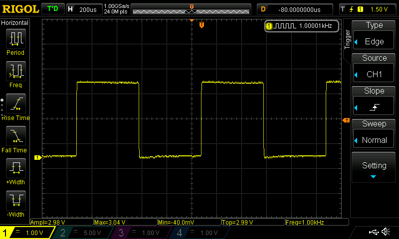
While the definition of bandwidth seems very straightforward, sometimes the application to common signals can be confusing. Consider an ideal square wave at 1 kHz. This signal repeats at a frequency of 1 kHz, so we might assume that it has a bandwidth of 1 kHz. In fact, an ideal square wave contains components at all odd multiples of the fundamental frequency, in this case at 3 kHz, 5 kHz, 7 kHz, etc. The practical upper limit, which determines the bandwidth of the signal, depends on how “ideal” the square wave is — in other words, the sharpness of the edges. While the amplitude of these components falls with increasing order, they’re important for properly constructing the original waveform. In fact, a common way to generate a sine wave is to filter out the higher-order components of a square wave signal.
Given a signal, how do we determine its bandwidth? The plain old telephone service (POTS) of my youth, for instance, passed frequencies between 300 Hz and 3000 Hz, which was found to be sufficient for voice communications; we might say signals passing through this system were limited to a bandwidth of 2700 Hz. While this would be true if the POTS system had sharp frequency edges, in reality, the signals passing through will have some small components below 300 Hz and above 3000 Hz. Because of this, it’s more common to define a non-zero threshold for the edges of the band. For instance, in measuring the highest and lowest frequencies in a signal, we might use the frequencies where the signal power is half of it’s peak value, or – 3 dB, corresponding to 70.71% in amplitude terms. While 3 dB is by far the most common value, you’ll find others used as well.
System Bandwidth
 A third use of the term bandwidth is to describe the range of frequencies passed by a system, such as a filter, amplifier, or the telephone system described above. While a particular signal passing through the system may have a quite narrow bandwidth — a nearly-pure sine wave at around 2600 Hz with a bandwidth of just a few Hz, for instance — the system itself still has a bandwidth of 2700 Hz. As with signal bandwidth, system bandwidth can be measured at 3 dB points (where the signals passed by the system have dropped to half power), or using other thresholds — 6 dB and 20 dB might be used for certain filters.
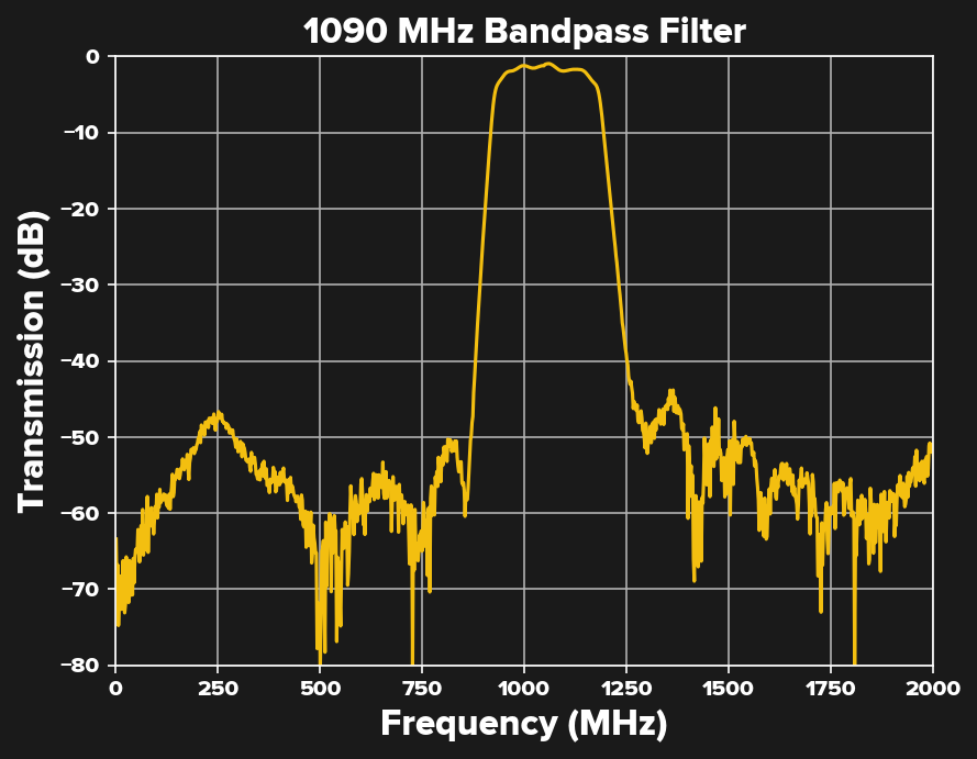
As an example, I measured the response of a 1090 MHz filter for receiving ADS-B transmissions. The 3 dB response of this filter extends from 927.3 MHz to 1,181.8 MHz, for a 3 dB bandwidth of 254.5 MHz. On the other hand, if measured at the -20 dB points, the filter has a 312 MHz bandwidth.
For another practical example, consider an oscilloscope — the “X MHz” in the scope specifications refers to the bandwidth, and this is almost always measured at the -3 dB point. The front-end amplifier of a 100 MHz oscilloscope will pass frequencies between 0 Hz (DC) and 100 MHz with 3 dB loss or less. This means that a 100 MHz sine wave may only show 71% of its actual amplitude, but also that frequencies somewhat above 100 MHz can be viewed — they’ll just be reduced in amplitude even more. The other consequence is that a 100 MHz square wave will look like a sine wave on a 100 MHz scope; to get an accurate picture of the square wave, the scope must have a bandwidth greater than about five times the square wave fundamental frequency. The 100 MHz oscilloscope is best used for observing square waves of 20 MHz or less.
Oscilloscope bandwidth is commonly assessed by measuring the rise time of a very fast edge. Assuming the signal edge is much faster than the rise time of the oscilloscope, the bandwidth of the scope is BW = 0.35/t_rise, with bandwidth in Hz and rise time in seconds. A scope with a rise time of 1 ns, for example, has a bandwidth of 350 MHz. The 0.35 factor assumes that the frequency-limiting elements in the scope’s front end produce a Gaussian filter shape, although the result is almost identical for a first-order RC filter; scopes with a sharper “brickwall” response may have factors of 0.45 or more. For more information about oscilloscope bandwidth, check out this article by Jenny List.
Information Capacity
At the beginning of this article, I mentioned a connection between digital bandwidth and signal bandwidth: it turns out that the relationship between them is a cornerstone of information theory. Consider the question of what you can do with a channel of 1 Hz bandwidth. What’s to limit the amount of information that can be sent over this link? Claude Shannon was the first to solve this problem for an abstract communication system where symbols are sent over the channel. He came up with the Noisy-channel coding theorem, which showed that the maximum possible information rate depends on probability that a symbol gets corrupted in transmission. Channels which create more errors during transmission limit the rate that data can be transmitted, no matter how clever we get with error-correcting codes.
Later, the Shannon-Hartley theorem extended this result to less abstract signal channels where the error is due to additive white Gaussian noise (AWGN). The net result is the same: it’s noise in the channel that ultimately limits the rate of information that can be transmitted. In the case a channel corrupted with AWGN, we have the following result.

The channel capacity, C, in bits/second, depends on the bandwidth, B, in Hz, and the ratio of the signal power, S, to the noise power, N, in the channel. This is the theoretical limit of the channel, and we may have to work very hard coming up with clever error-correcting codes to approach this limit in practice, but we can never exceed it.
Armed with this equation, we can return to the original question: how much information can we send over a 1 Hz channel per second? If the channel is noise-free, the signal-to-noise ratio (SNR) is infinite, and we can send data at an unlimited rate — of course, this never happens. In the case of equal signal and AWGN noise powers, or a 0 dB SNR, however, the result shows that we can only send a maximum 1 bit per second. That’s a big drop from infinity! On the other hand, if we have a channel of 60 dB SNR, we can theoretically send a maximum of 19.9 bps in our 1 Hz bandwidth. Of course, if the noise level remains the same, we need to increase the signal power by 60 dB — a million times — to achieve this. And, the reality is that we can only approach these rate limits, and the codes which do so comprise a large body of research.
Bandwidth = Bandwidth = Bandwidth
Even though the term is used in different ways in different contexts, the concepts of bandwidth are very simple. In a nutshell, signal bandwidth is the amount of frequency occupied by a signal, system bandwidth is the range of frequencies passed by the system, and digital bandwidth is the rate at which information flows over a channel. But, connecting these simple concepts are some very interesting fundamental principles of information theory. We’ve only been able to scratch the surface of this fascinating area in this article; sound off in the comments below if you’d like to see more articles about information theory.


You forgot one…
https://www.mcmaster.com/band-saw-blades
Missing that one, was not being kerful…..
I’ll get me coat…..
Your wit is cutting, but I saw it coming. Still, it was something I could sink my teeth into.
This is some cutting edge stuff…
You should probably include a comment in your section on O’scopes about sample rate on the scope. Your description of bandwidth is correct for an analog scope and correct for a digital sampling scope as long as you are far enough below the sample rate. When your input signal frequency starts getting close to about 1/5 of the sample rate, the analog front end bandwidth of the scope stops being the limiting factor.
good point, but that’s a whole other can of worms that probably doesn’t fit into these scant 1600 words. For instance, I have a scope with 20 GHz bandwidth and 200 kHz sample rate ;-)
perhaps another piece is in order
Ah, Bandwidths and its many meanings.
I almost have a hobby of confusing people in regards to it.
Though, then there is latency, shortened to “lag” and typically wrongly attributed to a lack of adequate bandwidth….
That bugs me sometimes. One of the fact based podcasts I listen to was talking about communication in private, so they covered something that was done in the far east: a slave’s head was shaved, tattooed with the private information, and the hair left to grow for a while, then they were transmitted. The group concluded that this was a low bandwidth communication mechanism, every time I hear this I scream (in my head) “it’s not low bandwidth, it’s high latency!!!”
sorry, how many GB of data were being encoded in the tattoo?
The classic example is a station wagon full of backup tapes. It’s high latency, and high bandwidth. It takes a while for the first data to get there, but once it arrives, the data moves quickly.
I guess the updated version would be a van full of microSD cards.
There is actually companies driving semi trailers full of hard drive arrays between datacenters.
Since one can then move tens/thousands of PB in a couple of hours.
(If one needs 2 hours to write the data to the array, 5 hours to drive it over to the other data center, and 2 hours to read it, and one has 10 PB of data, then one has an effective data rate of almost 2.5 Tb/s. (Reading and writing will though need to be done at 11 Tb/s, but this is a short distance.) Though, a semi trailer can carry far more then 10 PB of data….)
Wikipedia:
If an Airbus A380 were filled with microSD cards each holding 512 gigabytes of storage capacity, the theoretical total storage space onboard would be approximately 91 exabytes. A 4h47m flight from New York to Los Angeles would work out to a data transport rate of well over 5 petabytes per second, although this does not account for the time required to write to and read from the cards, which would almost certainly be much longer than the duration of the flight.
There was a story long time ago about an ISP claiming very fast DSL but wasn’t. Then a company suffering from slow Backups due to this pat the Backup onto a SD card wich was carried by a pigeon to the headquarters. That outperformed the DSL big time and was quite a story in the media.
https://winfuture.de/news,49721.html
Depending on the type of system, most “lag” is the result of either bottlenecks in the routing, or packet loss… but try to tell a customer that they are getting packet loss from trying to connect to an antiquated system from too far away…
I am also reffering to what most people think of as lag
Where o’ where have my packets gone?
Your packet hit a pocket on a socket on a port.
Yes, “lag” or stutter as I prefer to call it has a whole slew of reasons behind it.
Latency rarely being the actual reason. (Since latency is just a delay, it shouldn’t stutter due to it.)
But slew is a whole different kind of lag!
It has taken me way too long to partly understand your joke….
THIS!
I tire of the illiterate idiots who approach a latency problem with MOAR BANDWIDTH!
If the site is only reachable via a GeoSync satellite, having 500 MBPS of speed isn’t going to make a full back and forth transaction any faster.
Though, there are some applications where higher bandwidth can result in lower latency.
But that is when we have a low bandwidth bottleneck leading to queuing on either side of it.
But one can also have a high bandwidth link with far higher latency then a low bandwidth link, due to the higher bandwidth link would in this case send many piece of data in parallel at a lower clock rate compared to a more serialized buss. In the end, there are ups and downs at every turn….
Here’s another: in non-parametric statistics, the term bandwidth describes the width of the convolution kernel. Ahhhh, another fine term–convolution!
Convolution is quite a convoluted subject, wouldn’t you say?
And another: https://www.rubberband.com/about-us/rubber-bands-size-chart
That’s closely related to the bandsaw link posted above, though ironically, bandsaws are not particularly well-suited to cut rubber bands.
“Say It With Me: Bandwidth”
Baaannndddwwwiiddtthhh.
And now I can feel my IQ rising. ;-)
https://www.sciencedirect.com/science/article/pii/S0160289617302787#s0030
i always considered bandwidth an analog thing and prefer to use the term throughput for digital networks.
My AirFibre 5x link would agree with you.
It’s ok, I’m width the band
So “digital bandwidth” isn’t bandwidth at all, but the rate at which information is transmitted? Why not just call it that?
Throughput ?
that’s what i call it.
On IQ modulation a 1Hz lowpass has a 2Hz bandwidth because it extends to -1Hz :)
“Digital Bandwidth” is still directly tied to the frequency-domain. Most systems use a modulated analog carrier for data transmission, and those carriers exist at a frequency on the spectrum – yes, the digital information is carried on an analog medium with RF. For example, cable modems use QAM in NTSB countries at 6MHz signal bandwidths intended to fit within an NTSB signal channel’s bandwidth. QAM is a time-domain modulation that is places the “logic high” at different amplitudes at different times to form what is called a signal “constellation” in diagnostics; on a specialized scope it appears as a grid of dots of x dimensions, depending on the species of QAM, such as QAM64, QAM 256, etc.In this way a great amount of information can be transmitted in a very short period of time. Each “dot” in the constellation is a digital data point. Modern systems have multiple downstream(to the client device) channels and multiple upstream(return from the client device) channels simultaneously. You may notice that stuff comes down much faster than it goes up. There’s a physical reason for this. Upstream carriers are commonly in the HF or low VHF. The lowest I have seen was 26MHz. Downstream channels are usually placed in the VHF and UHF ranges. Most systems use about 1GHz for their channel plan, but 1.2GHz , 1.5GHz, and 2GHz systems exist, although transmission equipment such as coax, splitters, and connectors from the head end to the consumer need to be rated for these higher frequencies, as most common equipment is rated for 1GHz. Lower frequencies of a given bandwidth have a lower data rate capacity, or “symbol” rate aka “Baud”; but this measure has fallen out of favor for BPS or bPS, and when relating to signal efficacy, BER and MER which is tied directly to the SNR, or signal-to-noise ratio.
TLDR it’s an interesting topic to me and I’ve probably gone on too long here :p
I really appreciate your succinct explanation. I’m familiar with the topic and I still enjoy reading it. I’m sure more people than just myself would like to read more!
you can avoid throttling if you use a vpn. i tried surfshark and pure. pures cheaper cause they keep posting deals. right now they have a halloween campaign