
Anybody interested in building their own robot, sending spacecraft to the moon, or launching inter-continental ballistic missiles should have at least some basic filter options in their toolkit, otherwise the robot will likely wobble about erratically and the missile will miss it’s target.
What is a filter anyway? In practical terms, the filter should smooth out erratic sensor data with as little time lag, or ‘error lag’ as possible. In the case of the missile, it could travel nice and smoothly through the air, but miss it’s target because the positional data is getting processed ‘too late’. The simplest filter, that many of us will have already used, is to pause our code, take about 10 quick readings from our sensor and then calculate the mean by dividing by 10. Incredibly simple and effective as long as our machine or process is not time sensitive – perfect for a weather station temperature sensor, although wind direction is slightly more complicated. A wind vane is actually an example of a good sensor giving ‘noisy’ readings: not that the sensor itself is noisy, but that wind is inherently gusty and is constantly changing direction.
It’s a really good idea to try and model our data on some kind of computer running software that will print out graphs – I chose the Raspberry Pi and installed Jupyter Notebook running Python 3.
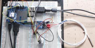
The photo on the left shows my test rig. There’s a PT100 probe with it’s MAX31865 break-out board, a Dallas DS18B20 and a DHT22. The shield on the Pi is a GPS shield which is currently not used. If you don’t want the hassle of setting up these probes there’s a Jupyter Notebook file that can also use the internal temp sensor in the Raspberry Pi. It’s incredibly quick and easy to get up and running.
It’s quite interesting to see the performance of the different sensors, but I quickly ended up completely mangling the data from the DS18B20 by artificially adding randomly generated noise and some very nasty data spikes to really punish the filters as much as possible. Getting the temperature data to change rapidly was effected by putting a small piece of frozen Bockwurst on top of the DS18B20 and then removing it again.
Although, for convenience, I derived data from a temperature sensor, a moving machine such as a robot would be getting data from an accelerometer and probably an optical encoder and a filter that updates ‘on the fly’ is essential.
Moving Averages
The simplest form is what’s called the ‘Simple Moving Average’ (SMA), which is similar to the weather station temperature example except that the 10 latest readings are updated with 1 fresh reading. Then, to make room for this new reading, the oldest reading is booted out. Since we’re coders and not mathematicians, the SMA can be best understood in code:
# SMA:
n = 10
array_meanA = array('f', [])
for h in range(n):
    array_meanA.append(14.0)         # Initialise the array with 10 values of '14'.
for x in range(n):
    getSensorData()                  # Get some data.eg tempPiFloat
    array_meanA[n] = tempPiFloat     # tempPiFloat slots into end of array.
    for h in range(n):
        array_meanA[h] = array_meanA[(h+1)]     # Shift the values in the array to the left
    meanA = 0
    for h in range(n):
        meanA = array_meanA[h] + meanA          # Calculate the mean, no weights.
    meanA = meanA/n
As can be seen, the code is fairly heavy on memory resources as it uses an array of floats. Nonetheless, it’s effectiveness can be improved further by adding weights to each value in the array such that the most current reading is given more prominence. The subsequent code is a bit more protracted and can be seen in the Jupyter Notebook file, but still entirely comprehensible! The filter would then be called a ‘Weighted Moving Average’ (WMA) and gives much less error lag with only a slight loss of smoothness, depending on the weights selected.
EWMA
If we feeling lazy and don’t want to clog up our memory with a large array of floats, we can use what is called an ‘Exponentially Weighted Moving Average’ (EWMA) which sounds pretty nasty but is actually incredibly simple:
# EWMF:
a = 0.20                  # Weighting. Lower value is smoother.
previousTemp = 15.0       # Initialise the filter.
for x in range(n):
    getSensorData()       # Get some data, eg tempPiFloat
    EWMF = (1-a)*previousTemp + a*tempPiFloat
    previousTemp = EWMF   # Prepare for next iteration.
Again, we don’t have to be a mathematician to see roughly what’s going on in the code above. With the weighting value ‘a’ set to 0.2, 20% weight is given to the current reading, and each previous reading effectively gets multiplied by 0.2 each additional period as time goes on. If we were to imagine that ‘a’ was our tuning knob, then the filter can be tuned for a particular application, with higher values of ‘a’ giving less error lag but more wiggliness. The only real disadvantage compared to the WMA is that we don’t have so much control over the weights. If you are inclined to, please have a look at the mathematical proof for EWMA.
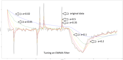
The graph below shows the EMMA filter in action with the DS18B20 and a piece of frozen German sausage. There are six different values of a, our tuning knob, and it should be possible to see the lag versus wiggliness tradeoff. I’d say that a value of a=0.2 gives best results on this rather spiky data.
There are of course hundreds of different filter algorithms to choose from, and they all have strengths and weaknesses. Both the simple and exponentially weighted moving averages are sensitive to large bogus values, or outliers. The simple average is only effected as long as the large value is in the moving window, but the EWMA sees the effect trailing off continuously, and perhaps slowly.
If you want a filter that’s immune to a few outliers, try the moving median filter. If you know a lot more about the dynamics of the system, a Kalman filter or similar first- or second-order filters might help, but at the expense of more calibration. I tried them on my temperature data, and they worked reasonably well but often gave unpredictable results such as over-shooting when the temperature suddenly stopped it’s decline. It was also pretty hard to initialise the filter and sometimes it would just shoot off into infinity!
One last thing that I really wanted to solve was to get a filter working for polar coordinates. The fact that degrees wrap around from 359° back to 0° makes a naive attempt at filtering difficult. If you simply average them together, you end up around 180°.
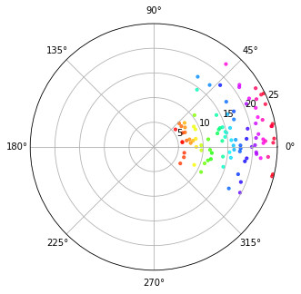
The answer was to convert the polar degrees to radians and then to a complex number. I simulated wind speed and wind direction using Gaussian noise in this Jupyter Notebook, and centred the data around 10° with a variance of 20º. Python handles the basic math required to calculate the mean wind direction seamlessly and there are also libraries available for MCUs such as Arduino to do the same thing.
Whenever you have real-world data input, it’s going to have some amount of noise. Dealing with that noise properly can make a huge difference in the behavior of your robot, rocket, or weather station. How much filtering to apply is often a matter of judgement, so starting off with a simple filter like the EWMA, plotting out the data, and adjusting the smoothing parameter by eye is the easiest way to go. When that fails, you’re ready to step up to more complicated methods.


Heat flow is non-deterministic. I wonder how that effects a predictor type filter like the Kalman? Anyway, Kalman filters have been used in any bit of moving ordinance with a processor since the Apollo Guidance Computer. IIRC all the drone flight software uses Kalman filters for navigation and flight dynamics. Even on little AVR’s. The hard part is in properly characterizing the expected behavior of a system.
Heat flow is deterministic. You cannot simply call systems which you don’t understand as non-deterministic.
For the love of $deity.
Sensor filters for _coders_. Really?
it’s python, no need to copy the whole fricken array every iteration. Just
array_meanA.append(tempPiFloat)
array_meanA.pop(0);
Not that it would make any more sense in c or any other language where you would just insert every new element at a rotating index:
array_mean[i] = tempPiFloat;
i = (i + 1) % n;
And if you bloody _must_ copy data around, at least do it in a pythonic way.
array_meanA[0:n-1] = array_meanA[1:n]
And the provided mean calculation is just ugly.
meanA = sum(array_meanA)/n
By the way, despite Python is not for performance, if the array is large the sum of the whole array could be avoided too:
mean = mean – array[i]
array[i] = sample() / n
mean = mean + array[i]
i = (i + 1) % n
Is this article somebodies first program or something? Who has never used python before?
python being used by people who know what they are doing isn’t too bad (though I don’t like some of it’s design decisions) however this type of program reminds me of some of the crap written in those early BASICs by people who really had no idea…
Not a coder/programmer myself I don’t know good code from bad. Could you explain what is the problem with this code and how could
It be made easier to understand the concept?
Mostly what JR said.
Whatever the language you use, learn it’s built-in functions.
Just to pick an example, Python provides a “sum()” function. Using it will be more efficient than implementing it yourself using a for loop.
There is a lot of things going under the hood, even more with high level language like Python. Aside for memory or computational benefits of using built in library, most of the time, coding your function will lead to edge case that are already ironed out and optimized by the lib.
It’s not always the case, and you may need to use extern library when you need a lot of processing power.
But for entry level coding, like this lovely moving average function,
”
average = sum( values ) / len( values )
”
is much more understandable (and faster, and memory efficient) than
”
meanA = 0
for h in range(n):
meanA = array_meanA[h] + meanA
meanA = meanA/n
”
Honestly, you won’t gain much performance in this articular case.
But start working with thousands of values / objects, and you will need to use iterators or I don’t know what is relevant to your project.
Most of the time, the best optimizations are achieved by changing your algorithm.
For example, instead of copying your array to change the first value with a new one, just use a rolling index, it uses more memory (one index) but saves you the “copy each value to it’s predecessor’s place” time.
As for the article itself, it’s nice.
Maybe could it talk a bit about other representation to better filter things out (like frequency domain or so), but I digress.
Sorry, I wrote a wall again…
I tought Python IS (or was) actually used in various places/labs for maths and multiple dimension arrays operations for performance and ease of coding. Of course using libs in C/C++ binary compiled for the platform.
Yes, Python is used a lot in HPC (High Performance Computing), but as _interface_ to the real HPC libraries (written usually in C/C++ or directly implemented in hardware). Is like like a “better shell scripting”, but the heavy duty work its done by something that usually is not written in Python. It is also very useful, since HPC is needed in areas where numeric computation is quite demanding and complex, so the users are usually experts in their scientific/engineering areas but _not_ in low level languages like C/C++. In these languages you can (if you use them properly, which is not easy) have better usage of the raw resources of the machine. So, one popular approach is to use Python as interface of a library, and the main math algorithms that can be invoked millions of times to be implemented in C/C++ or even assembler. Common and heavy math operations (like matrix multiplication, etc) usually go directly in hardware (like GPU/FPGA).
Hence, Python, despite having an important role in HPC, is not considered a high performance language on its own, and performance is not its main focus but usability (very important to be used as interface!).
The sample code is really messy and inconsistent. For a demonstration all article it’s probably best to clean it up a bit. E.g. Consisten code style (flake8 can help here), undefined variables (n for example). Why is get sensor data not simply returning the data, rather then putting it in a global, etc etc. this small changes would make the code far easier to read and would not teach readers bad practices.
This is really cool. Years ago I spent some time trying to come up with a good way of taking a weighted average of a rotary encoder output and never came up with anything that wasn’t a total bodge, and this is a neat hint as to how I should have done it.
the one euro filter is a nice solution for smoothing data whilst not being as laggy as the moving average types
http://cristal.univ-lille.fr/~casiez/1euro/
and for filtering angular data simply convert to cartesian coordinates apply filter of choice to each axis and convert back to an angle
an example can be found in the utils.c of the vesc firmware
https://github.com/vedderb/bldc/blob/master/utils.c#L210
Why not just add 360n or 2pi and average those? Subtract on the way out.
Averaging filters are dumb, unresponsive, and way too linear. I wish I could post my favorite….
I recall many years back working at a university, we were doing an experiment and had a transducer that has a cyclic output that was buried in noise. I went the electronics route and developed a sharp active filter at the cyclic frequency, while a coworker went to the math department and teamed up with a very smart guy and came up with a digital approach.
My system worked so so, it had the pitfalls you would expect as far as delay and bad step response. Lucky for us, these were not big deals in this case.
The digital system was amazing. We got beautiful data out of the system. Or so we thought. One day I had the data acquisition system on and running before I turned the servo hydraulic system on, so there was no physical input to the sample, and the digital system was STILL pulling nice looking data out of the noise.
There are a lot of both analog and DSP techniques that can be used, but you have to be careful in their application. Sometimes beyond the obvious.
The best way to filter a wrapping number system (such as polar degrees) is to simply add a positive offset to it, filter it normally, then remove the offset. For the polar angles, just add another 360 (or 1000 for all it matters), then filter, then subtract the offset again. None of this silly coordinate conversion is needed. Save yourself some CPU cycles for goodness sake.
That’s a great solution! Not thought of that.
that doesn’t work .
you are wanting to average the values across the boundary ie .. noise of +- 10 around 0 should filter to zero not 180 which is what your scheme does
its not saving cycles if it doesn’t work!
It does work: 0±10 values become 1000±10, which do average to 1000, and then you subtract that offset.
Take care to keep the data from hitting the actual machine precision limits while it’s offset — ie, 2**15 for signed 16-bit, etc, so don’t go adding 32000 to it as an offset in that case, although you could if you can keep it as unsigned 16 bits (max value, 2**16-1 before adding one more will overflow to zero again).
l could be misunderstanding, but i still see that failing to account for the boundary, lets work in degrees to ensure we are on the same page and that 360 and 0 are equivalent.
angle1 = 0 + 10 = 10
angle2 = 0 – 10 = 350 // this is why offsetting wont work
add offsets
angle1 = 1010
angle2 = 1350
mean angle with offsets = (1010+1350)/2 = 1180
remove offsets = 180
which is as far away as you can be from the desired result. as noted its the wrapping that causes the failure and i dont see how to get away from that by shifting
if anyone can talk me through or link to some functional code. that would be ace
I’d be happy to explain in more detail how to code for polars. As you said above, the offset idea does not work :( …… Check out https://github.com/paddygoat/Kalman-Filters/blob/master/Polar_Wind_Direction.ipynb for my crappy, but functional, python code.
You’re adding the offset too late.
ang1 = 10 + 1000 = 1010
ang1 = -10 + 1000 = 900
Mean = 1010+900 = 2000
Mean/2 = 1000
Remove offset = 0
It does not work when the difference between the two angles is over half a circle. For example for 179 and -179 (almost a full circle).
ang1 = 179 + 1000 = 1179
ang1 = -179 + 1000 = 821
Mean = 1179+821 = 2000
Mean/2 = 1000
Remove offset = 0
… but it should be +180 (or -180)
If you want your averages around 0, you need your numbers to be relative to 0. Your solution doesn’t work because you’re saying 10 degrees below 0 is 350 – you need to call it -10, as TT does.
Basically, you need to think about what you’re measuring, and what you need to work out. They need to be in the same format, with the same reference point.
Thought about this some more, from half baked earlier. You can’t average -ve numbers with positive. Add 360 to each -ve angle so the angles are all in a 360 range of positive numbers.
have a look a benjamin vedders bldc utils to see a decent implementation
https://github.com/vedderb/bldc/blob/master/utils.c#L210
and the one euro filter is nicer than the exponential moving average for many purposes
http://cristal.univ-lille.fr/~casiez/1euro/
That’s a funny filter. It’s an EWMA with a smoothing parameter that depends on the distance between the last value and the running mean. (I didn’t / couldn’t read the paper, but I read the filter implementation in code.)
Whether that’s better or worse depends on your data, though… For their use case, it looks like they’re trying to track a finger on a touchscreen. There, you’d expect long periods of dwelling at a single value (where less weight on the current value is good) followed by quick, continuous movements (more weight on the current value is better).
But imagine that you’re trying to filter out measurement error in a relatively static/slow process. Then the “adjustment” to lower smoothing b/c you got a far-off value makes the filter do less filtering, which could be worse than a static EWMA. The 1€ filter adapts to become more sensitive to noise after it has seen an outlier.
In other words — the authors seem to have a specific data-generating-process in mind, and they’re tailoring their filter to that. For such cases, an old-school stats guy would recommend a Kalman or similar filter.
I wouldn’t use the 1€ filter on a thermometer, for example. But it might exhibit lower lag on a touchscreen (for a given jitter when not moving).
So yeah — what you said. :) Might be better than a simple EWMA for some purposes. At the expense of another parameter to calibrate and some more computation.
An EWMA filter has the same effect as a low pass RC filter and you can calculate the RC time constant if you know the loop frequency of the code (and the weighting).
If you need a lot of smoothing at low amount of RAM & processing time, CIC filter is a good choice: https://en.wikipedia.org/wiki/Cascaded_integrator%E2%80%93comb_filter
Its response is roughly same as a gaussian blur filter, but with logarithmic amount of memory vs. blur length
A computationally efficient sliding window filter:
Fn = (Current_Sample + Fn-1) / 2.
The division can be implemented as a right shift. The window length is the effective number of bits being used. No need to store a window’s length of data either. Good for simple data smoothing.
This is EWMA with a=0.5 — it’s fairly responsive to the present value / noise.
But the general point, for constrained systems, is great. I do EWMAs with power-of-two divisors on AVRs (for instance) to take advantage of the bit-shift division.
There’s other tricks that are relevant for integer math, like getting the rounding right and calculating 15/16 efficiently, but that’s a whole ‘nother can of worms.
Hmmmm…I seem to remember learning about IIR and FIR digital filters and their implementation algorithms a very long time ago…as in the 1980s. How come zero mention of these canonical filter types and their uses, even as just amusements around odd rotating-buffer tricks. I would assume there’s by now even good software for synthesizing them. No?
If you’ve access to MATLAB, the Filter Designer in the Signal Processing Toolbox is a darned quick way to noodle with FIR & IIR filters. Though, in a pinch, Excel can be pressed into service for it too (hint: the Analysis Toolpak has a FFT tool). But I’m sure without even looking that there are many web-based calculators that can help you out too.
I like me the part with the Bockwurst
Comments on spelling or grammar in a technical forum piss me off much more, really.
They leave the bitter “why fuck did I just read” taste.