[Paul Curtis] over at Segger has an interesting series of blog posts about calculating division. This used to be a hotter topic, but nowadays many computers or computer languages have support for multiplication and division built-in. But some processors lack the instructions and a library to do it might be less than ideal. Knowing how to roll your own might allow you to optimize for speed or space. The current installment covers using Newton’s algorithm to do division.
Steve Martin had a famous bit about how to be a millionaire and never pay taxes. He started out by saying, “First… get a million dollar. Then…” This method is a bit like that since you first have to know how to multiply before you can divide. The basic premise is twofold: Newton’s method let you refine an estimate of a reciprocal by successive multiplications and then multiplying a number a reciprocal is the same as dividing. In other words, if we need to divide 34 by 6, you could rewrite 34/6 to 34 * 1/6 and the answer is the same.
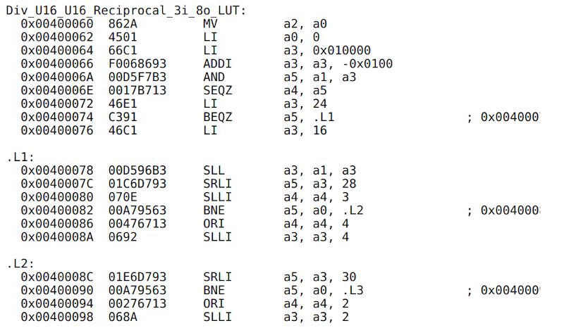
Newton’s approximation for reciprocals lets you take a guess at the answer and then refine it through a series of multiplications. Each multiplication creates better accuracy. You can use this to perform a classic speed/space trade-off. For example, let’s just assume we want to find the reciprocal of a byte (presumably a fixed point byte). A look-up table of 256 elements would provide perfect accuracy and would be very fast. No more math is necessary. But what about 32 bits? Now the table is just too big. But you could look up, say, the first 8 bits of the 32-bit number. Or more. Or less. Depends on what’s important to you.
So now you have a poor estimate of your reciprocal. Sir Issac can make it better. For some number a, You take your estimate (x) and multiply them together. Subtract that number from 2 and you have a factor to multiply your old estimate by to get a new estimate. Skipping ahead, it is clear if your estimate was right, the multiplication would give you 1 which would not change the old estimate at all. If the estimate is off, you’ll get a scaling factor.
As a formula it looks like this:
x=x*(2-a*x);
So if you decide the reciprocal of 22 might be .02, the first pass will give you:
0.02*(2-22*0.02) = .0312

.0312*(2-22*.0312) = .0410

.0410*(2-22*.0410) = 0.0450
The right answer is a repeating decimal 0.0454545 and if you keep going, you’ll get there.
Of course, then you have to multiply one more time to do the division.
We liked that the post has a fixed-point implementation and then examines the resulting assembly code for ARM, RISC-V, and dsPIC30. Well worth a read.
We love math tricks we can use in assembly language. If you are working on AVR and floating point, don’t miss this method.


“… if we need to divide 34 by 6, you could rewrite 36/6 to 36 * 1/6 and the answer is the same.”
I hope that is a typo, because 34/6 != 36/6 (the difference is statistically significant, too).
US customary units?
No – scalar and dimensionless. It is pure arithmetic.
36/6 = 6
34/6 = 5.6666 … … … 67
The US isn’t uncustomed to creating their own scalars. They almost has pi = 4!
“4!” but that’s wrong by nearly 21
The actual number we almost had it equal to in ONE state was 3.
It’s well-known crackpot Miles Mathis who asserts that pi = 4.
http://milesmathis.com/pi7.pdf
“Facts are stupid things.”
Pi is exactly 10.
In base-pi.
I did some research into this. The “geometric simplification act” redefining pi as 3 actually came from a satirical article, so that did not actually happen. However, there was the 1897 “Indiana Pi Bill”, where an amateur mathematician almost convinced the state to put one of his crazy math ideas into law. He did not specifically mention pi in his proof, but a consequence of his ideas was that pi would be defined as exactly 3.2.
https://en.wikipedia.org/wiki/Indiana_Pi_Bill
Just remember that there is a non-integer number base where the value of pi is precisely written as a single digit, 3.
Probably fluid ounces.
Nano parsecs per micro fortnight?
At least it isn’t firkins.
In integer math, it is the same, depending on the rounding rules.
If you aren’t dividing by shifting right a fixed number of digits then are you even a programmer? ;)
Bitshifting 1 position will always divide/multiply by 2.
For n-positions, it is by 2^n.
This doesn’t work with numbers that are being represented as a floating point number, as those are just weird. (Because of the mantissa and exponent.)
That’s the joke.
You nailed it.
You sure did an understanding.
Ah, I implemented this a lot of years ago (the Newton-Raphson method) on Texas Instruments C5000 assembly language and was amazed at how well it performed. This technique is specially useful when you have to divide a lot of numbers by the same divisor: you compute the reciprocal once and then just multiply every number by it. On machines with hardware multiplication (like the aforementioned DSP family) this runs blazingly fast.
If you do not have fast hardware multiplication, you can also fallback to the good old CORDIC division…
“you could look up, say, the first 8 bits of the 32-bit number….”
Make sure you get your table right, otherwise you end up with the Pentium division problem.
But wasn’t the 80×87 FPU 80-Bit wide?
Sure, it had an optional lower precision mode, but internally.. 80-Bits.
No, you do not need to get the table right. This method just uses the value from the table as an initial estimate. If the estimate is good you get a precise result after few iterations. If the estimate is bad it takes a few more iterations. Only problem is if your initial estimate was to big and the next estimate turn negative. But this is easy to detect and you can try again with a smaller initial estimate (for example by shifting it one bit). So even when your table is completely wrong you get good results.
Please don’t write “x=x*(2-a*x);”, that hurts badly !
rather something like x2 = x1 * (2-a*x1), or xn, or even better x_n for latex afficionados.
x *= (2 – a*x)
Yes, at least it’s an assignement.
Starting back in 1988, I developed some critical embedded system software for an Instrument Landing System (ILS). Both signal generation and monitoring had to be done with a 16 bit Intel 80C196KB microcontroller that had both HW multiply and divide. But its divide was MUCH slower, so I chose not to use its divide for speed reasons and because I designed the system to preclude its use since doing any fixup for division underflow was too expensive in code and time. How did I avoid divisions? By using reciprocals, but within tight limits. I retweaked the ILS signal generation HW to ensure that the desired signal generated by the system was always larger than I needed it to be (based on HW chip specs and a pad), so that less-than-unity calibration “gains” would always work for each system. A similar approach was also used for ILS signal monitoring (of a detected AM signals of several sample points of the navigation signal-in-space) calibrations, but that portion was redesigned to allow the AC+DC detected AM signal to be DC offset and gain adjusted “before” applying a FFT (actually, two Goertz transforms to capture the 90 and 150 Hz ILS signal components). Strict adherence to these rules insured that the system operated in spec and wouldn’t cause crashes.
Here’s the part you’re waiting for: To simplify the operations used, calibration gain (attenuation) of signals used a 16 x 16 bit multiply to generate a 16:16 result (i.e. 32 bits with a LS 16 bits being the “remainder”). The signals were always positive as were the gains, so I didn’t have to worry about 2’s complement overflow and always had nearly a full 16 bit dynamic range (except for its inherent attenuation). Rounding was easy, since all that was needed was to check the MS bit of the remainder and if set, I would increment (add 1) to the quotient (the MS 16 bits of the product).
I used a Newton-Raphson 16 bit square-root routine to calculate the Fourier magnitudes from the 32 bit product of multiplying the two 16 bit Fourier coefficients.
It’s all magic.