The Calculus is made up of a few basic principles that anyone can understand. If looked at in the right way, it’s easy to apply these principles to the world around you and to see how the real world works in their terms. Of the two main ideas of The Calculus — the derivative and the integral — today we’ll focus on the derivative.
You can enjoy this article by itself, but it is also worth looking back at the previous installment in this series. We went over the history of The Calculus and saw how it arose from two paradoxes put forth by a 4th century philosopher named Zeno of Elea. These paradoxes lead to the derivative/integral ideas that revolutionized mankind’s understanding of motion.
“Everything should be made as simple as possible, but not simpler.”
Albert Einstein
Our journey begins with a fictitious character whom we shall call [John Doe]. He represents the average professional worker who can be found in cities and towns across the world. Most everyday, [John] wakes up to his alarm clock and drives his car to work. He takes an elevator to his office and logs on to his computer. And he does these things without the slightest clue of how any of them work. While he may be interested in learning about the inner workings of the machines and devices he uses on a daily basis, [John] does not have the time and energy to invest in doing so. To him cars, elevators, computers and alarm clocks are completely different and complicated machines with hardly any similarities. It is simply not possible to understand how each of them work without years of study.
The regular readers of Hackaday might see things a bit differently than our [John Doe]. They would know that the electric motor that moves the elevator is very similar to the alternator in his car. They would know that the PLC that controls the electric motor that moves the elevator is very similar to the computer he logs in to. They would know that on a fundamental level, the PLC, alarm clock and computer are all based on relatively simple transistor theory. What is a vast complicated mess to [John Doe] and the average person is nothing but the use of simple mechanical and electrical principles to the hacker. The complication resides in how those principles are applied. Abstracting the fundamental principles from complicated ideas allows us to simplify and understand them in a way that pays homage to Einstein’s off-the-cuff advice, quoted above.
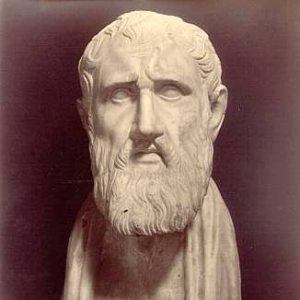
Zeno of Elea 490 – 430BC
Many of you look at The Calculus the same way [John Doe] looks at machines. You see the same vast, complicated mess that would require a great deal of time and effort to understand. But what if I told you that calculus shares a commonality in much the same way many different machines do. That there are a few basic principles that anyone can understand, and once you do, it will unlock a new way of looking at the world and how it works.
The average calculus course book is a thousand pages long. The [John Does] of the world will see a thousand difficult things to learn. The hacker, however, will see two basic principles and 998 examples of those principles. In this series of articles, I’m going to show you what these two principles – the derivative and the integral – are. Based on work done by Professor [Michael Starbird] of The University of Texas at Austin for The Teaching Company, we’ll use everyday examples that anyone can understand. The Calculus reveals a particular beauty of our world — a beauty that arises when you’re able to view it dynamically as opposed to statically. It is my hope to give you this view.
Before we get started, it pays to understand a little of the history of how The Calculus came about, and how its roots lie in the very careful analysis of change and motion.
Zeno’s Paradox
Zeno of Elea was a philosopher in the fourth century BC. He posed several subtle but profound paradoxes, two of which would eventually give rise to The Calculus. It would take over 2,000 years for man’s ingenuity to solve the paradoxes. As you can imagine, it wasn’t easy. The difficulties largely revolved around the idea of infinity. How do you deal with infinity from a mathematical perspective? Sir Isaac Newton and Gottfried Leibniz would go on to independently invent The Calculus in the mid 17th century, finally putting the paradoxes to rest. Let us take a close look at them and see what the fuss was all about.
The Arrow
Consider the arrow flying through the air. We can say with reasonable and competent assurance that the arrow is in motion. Now consider the arrow at any given instant in time. The arrow is no longer in motion. It is at rest. But we know the arrow is in motion, how can it be at rest! This is the paradox. It might seem silly, but it’s a very challenging concept to deal with it from a mathematical point of view.
We’ll find out later that what we’re really dealing with is the concept of an instantaneous rate of change, which we will elaborate on with the idea of one of the two principles of calculus – the derivative. It will allow us to calculate the velocity of the arrow at an instant in time – a monumental feat that took over two millennia for mankind to reach.
The Dichotomy
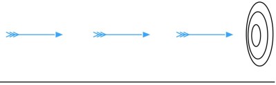
Let us consider the same arrow again. This time let’s say the arrow is coming at us. Zeno says we don’t have to move, because it can never hit us. Imagine that as the arrow is in flight, it has to cover half the distance between the bow and the target. Once it reaches the half way point, it has to do this again – move half the distance between it and the target. Imagine that we keep doing this. The arrow is constantly moving halfway between its origin and target. By doing this, the arrow can never hit us! In real life, the arrow does eventually hit the target, leaving us with the paradox.
As with the first paradox, we’ll see how to resolve this issue with one of the two principles of calculus – the integral. The integral allows us to deal with the concept of infinity as a mathematical function. It is an extremely powerful tool to scientists and engineers.
The Two Principles of Calculus
The two main ideas of The Calculus will be demonstrated by using them to solve Zeno’s paradoxes.
The Derivative – The derivative is a technique that will allow us to calculate the velocity of the arrow in “The Arrow” paradox. We will do this by looking at positions of the arrow through incrementally smaller amounts of time, such that the precise velocity will be known when the time between measurements is infinitely small.
The Integral – The integral is a technique that will allow us to calculate the position of the arrow in the Dichotomy paradox. We will do this by looking at velocities of the arrow through incrementally smaller amounts of time, such that the precise position will be known when the time between measurements is infinitely small.
It’s not difficult to notice some similarity between the derivative and integral. Both values are calculated by examining the arrow with increasingly finer time intervals. We will learn later that the integral and derivative are in fact two sides of the same ceramic capacitor.
Why Should I Learn Calculus?
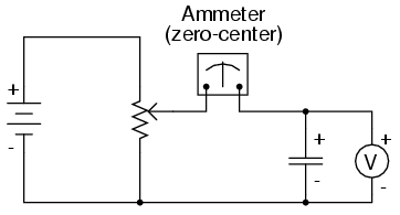
We are all familiar with Ohm’s Law, which relates current, voltage and resistance in a simple equation. However, let us consider “Ohm’s Law” for a capacitor. A current flow through a capacitor is dependent on the voltage across it and time. Time is the critical variable here, and must be taken into account in any dynamic event. Calculus lets us understand and measure how things change over time. In the case of a capacitor, the current through it is equal to the capacitance multiplied by volts per second, or: i = C(dv/dt) where:
i = current (instantaneous)
C = Capacitance in Farads
dv = change in voltage
dt = change in time
In this circuit, there is no current flow through the capacitor. The volt meter will read the battery voltage and the ammeter will read zero amps. So long as the potentiometer is not moved, the voltage on the meter will be steady. Our equation would say that i = C(0/dt) = 0 amps. But what happens when we adjust the potentiometer? Our equation says there will be a resulting current flow in the capacitor. This current flow will be dependent on the rate the voltage changes, which is tied to how fast we move the potentiometer.
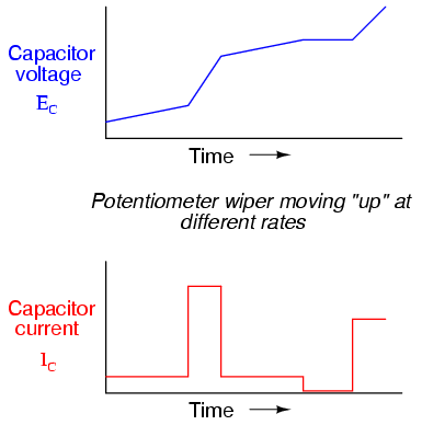
These graphs show the casual relationships between the voltage across the capacitor, the current through the capacitor and the speed we turn the potentiometer. It starts with the potentiometer turning slowly. An increase in speed results in a faster changing voltage which in turn results in a dramatic increase in current. At all points, the current through the capacitor is proportional to the rate of change of the voltage across it.
Calculus, or more specifically the derivative, gives us the ability to quantify this rate of change, so that we can know the exact value of current running through the capacitor at any given instant in time. The same way we can know the instantaneous velocity of Zeno’s arrow. It is an incredibly powerful tool to have in your hacking arsenal.
In the next article, we will go into deep detail of how we calculate the derivative using a modern but still simple representation of Zeno’s “The Arrow” paradox and some basic algebra. A following article will do the same for the integral using the Dichotomy paradox. Then we will tie things up by showing how the two are related, something known as The Fundamental Theorem of Calculus.
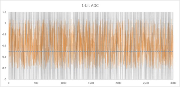
It’s a counterintuitive result that you might need to add noise to an input signal to get the full benefits from oversampling in analog to digital conversion. [Paul Allen] steps us through a simple demonstration (dead link, try Internet Archive) of why this works on his blog. If you’re curious about oversampling, it’s a good read.
Oversampling helps to reduce quantization noise, which is the sampling equivalent of rounding error. In [Paul’s] one-bit ADC example, the two available output values are zero volts and one volt. Any analog signal between these two values is rounded off to either zero or one, and the resulting difference is the quantization error.
In oversampling, instead of taking the bare minimum number of samples you need you take extra samples and average them together. But as [Paul] demonstrates, this only works if you’ve got enough noise in the system already. If you don’t, you can actually make your output more accurate by adding noise on the input. That’s the counterintuitive bit.
We like the way he’s reduced the example to the absolute minimum. Instead of demonstrating how 16x oversampling can add two bits of resolution to your 10-bit ADC, it’s a lot clearer with the one-bit example.
[Paul’s] demo is great because it makes a strange idea obvious. But it got us just far enough to ask ourselves how much noise is required in the system for oversampling to help in reducing quantization noise. And just how much oversampling is necessary to improve the result by a given number of bits? (The answers are: at least one bit’s worth of noise and 22B, respectively, but we’d love to see this covered intuitively.) We’re waiting for the next installment, or maybe you can try your luck in the comment section.
You may know your way around the registers of that favorite microcontroller, but at some point you’ll also need to wield some ninja-level math skills to manage arrays of data on a small device. [Scott Daniels] has some help for you in this arena. He explains how to manage statistical calculations on your collected data without eating up all the RAM. The library which he made available is targeted for the Arduino. But the concepts, which he explains quite well, should be easy to port to your preferred hardware.
The situation he outlines in the beginning his post is data collected from a sensor, but acted upon by the collection device (as opposed to a data logger where you dump the saved numbers and use a computer for the heavy lifting). This can take the form of a touch sensor, which are known for having a lot of noise when looking at individual readings. But since [Scott] is using the Mean and Standard Deviation to keep running totals of collected data over time it is also very useful for applications like building your own home heating thermostat.
As an HVAC engineer by trade, [Carlos Paris] spends a lot of time in AutoCAD designing all those hidden pipes, tubes, and ducts hidden in a building’s rafters. One day, [Carlos] read of an open contest – the prize was over a million dollars – to generate a prime number with a billion digits. [Carlos] misheard this as, ‘a prime number greater than one billion’ and of course said this was a trivially easy task and opened up his favorite tool – AutoCAD – in an effort to discover the largest prime ever. [Carlos] never generated a remarkably large prime, but he did come up with a very, very cool visualization of prime numbers on a number line, as well as a great justification of the twin prime conjecture, a problem in mathematics that has remained unsolved for several generations.
[Carlos] started his investigations into the properties of prime numbers by drawing a series of circles on a number line in AutoCAD. These circles were of diameters of all the integers, and going down the number line, these circles started to have an interesting, chaotic pattern (see above picture). [Carlos] found that whenever two circles intersected, that position was a prime number. It’s really nothing more than a Sieve of Eratosthenes, but it’s a very cool-looking visualization nonetheless.
Looking deeper into his graph, [Carlos] discovered there were certain primes that had another prime number just two places down the number line. For example, the numbers 3 and 5, 29 and 31, and 41,and 43 are twin primes, as the difference between the primes is only 2. The idea there are infinitely many twin primes is a famous unsolved problem in mathematics – it’s obvious it must be true, but no mathematician has yet come up with a proof of this conjecture.
[Carlos] looked at his number line and simplified it to a generic prime number. By taking a generic number line and overlaying the multiples of other prime numbers on this graph, [Carlos] had a very, very clever way of understanding exactly how twin primes come into existence.
In the end, [Carlos] is no closer to proving the twin prime conjecture than anyone else. We’ve got to hand it to him, though, for nerding out with an engineer’s favorite tool – AutoCAD – and managing to derive some fairly obscure mathematics on his own.
After the break you can see [Carlos]’s videos describing the though process that went into his creation. Very, very cool work.
[Michail] needed a new graphics card. The only problem was his motherboard didn’t have any free PCI-E x16 slots available. Unable to find a PCI-E x1 card, he did what any of us would do and broke out the Dremel. Yes, he got it working, but don’t do this unless you know what you’re doing.
It’s recycling!
[Steve] recently got a Galaxy S3 and was looking for something to do with his old phone. It’s got WiFi, it’s got a camera, and with a free app, [Steve] now has an IP Webcam. Neat way to recycle a phone.
Remember [Fredzislaw100], the guy who puzzled the Internet with impossible circuits? He’s back again, this time with wireless LEDs. We’re guessing something similar to an induction charging system in the battery clip, wirelessly coupled to something under the paper, and that is wirelessly coupled to the LEDs. Your guess will probably be better than ours, though.
Not shown: Captain Obvious, Major Major
Pv2 [Zachary Ricks] of the U.S. Army thought we would get a kick out of the last name of one of the guys in his company. Yes, it’s ‘Hackaday,’ and yes, it’s a real surname. Here’s the full pic [Zach] sent in. Apparently it’s a name along the lines of ‘Holiday.’ Honestly, we had no idea this was a real surname, but we’re thinking Private Hackaday could use a care package or two (dozen).
Anyone up for sending a few hacker friendly (for [Zach] and a few other guys) care packages? Even socks or books or Oreos would make for an awesome care package. Email me if you want the mailing address.
In August, 2010, [Alexander Yee] and [Shigeru Kondo] won a respectable amount of praise for calculating pi to more digits than anyone else. They’re back again, this time doubling the number of digits to 10 Trillion.
The previous calculation of 5 Trillion digits of Pi took 90 days to calculate on a beast of a workstation. The calculations were performed on 2x Xeon processors running at 3.33 GHz, 96 Gigabytes of RAM, and 32 Terabytes worth of hard drives. The 10 Trillion digit attempt used the same hardware, but needed 48 Terabytes of disk to store everything.
Unfortunately, the time needed to calculate 10 Trillion digits didn’t scale linearly. [Alex] and [Shigeru] waited three hundred and seventy-one days for the computer to finish the calculations. The guys used y-cruncher, a multithreaded pi benchmarking tool written by [Alex]. y-cruncher calculates hexadecimal digits of pi; conveniently, it’s fairly easy to find the nth hex digit of pi for verification.
If you’re wondering if it would be faster to calculate pi on a top 500 supercomputer, you’d be right. Those boxes are a little busy predicting climate change, nuclear weapons yields, and curing cancer, though. Doing something nobody else has ever done is still an admirable goal, especially if it means building an awesome computer.

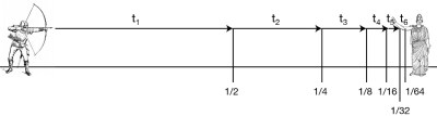 Let us consider the same arrow again. This time let’s say the arrow is coming at us. Zeno says we don’t have to move, because it can never hit us. Imagine that as the arrow is in flight, it has to cover half the distance between the bow and the target. Once it reaches the half way point, it has to do this again – move half the distance between it and the target. Imagine that we keep doing this. The arrow is constantly moving halfway between its origin and target. By doing this, the arrow can never hit us! In real life, the arrow does eventually hit the target, leaving us with the paradox.