Even for those of us that are quite technically minded, we spend precious little time thinking about the cables that carry our signals and do all the important work we need them to do on a daily basis. A great deal of theory and engineering goes into making things like telephone lines and HDMI cables work, but we mostly just plug them in and get on with whatever we’re doing.
If this is your experience, you might find the Hackaday Europe talk from [Michael Wiebusch] to be particularly interesting. He dives into transmission line theory from an accessible standpoint, explaining how two disparate signals can go in opposite directions on the very same wire. Then he demonstrates the theory by building a cable modem… well, sort of!
PCB design starts off being a relatively easy affair — you create a rectangular outline, assign some component footprints, run some traces, and dump out some Gerber files to send to the fab. Then as you get more experienced and begin trying harder circuits, dipping into switching power supplies, high speed digital and low noise analog, things get progressively more difficult; and we haven’t even talked about RF or microwave design yet, where things can get just plain weird from the uninitiated viewpoint. [Robert Feranec] is no stranger to such matters, and he’s teamed up with one of leading experts (and one of this scribe’s personal electronics heroes) in signal integrity matters, [Prof. Eric Bogatin] for a deep dive into the how and why of controlled impedance design.
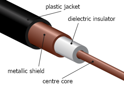
RG58 cable construction. These usually are found in 50 Ω and less commonly these days 75Ω variants
One interesting part of the discussion is why is 50 Ω so prevalent? The answer is firstly historical. Back in the 1930s, coaxial cables needed for radio applications, were designed to minimize transmission loss, using reasonable dimensions and polyethylene insulation, the impedance came out at 50 Ω. Secondarily, when designing PCB traces for a reasonable cost fab, there is a trade-off between power consumption and noise immunity.
As a rule of thumb, lowering the impedance increases noise immunity at the cost of more power consumption, and higher impedance goes the other way. You need to balance this with the resulting trace widths, separation and overall routing density you can tolerate.
Another fun story was when Intel were designing a high speed bus for graphical interfaces, and created a simulation of a typical bus structure and parameterized the physical constants, such as the trace line widths, dielectric thickness, via sizes and so on, that were viable with low-cost PCB fab houses. Then, using a Monte Carlo simulation to run 400,000 simulations, they located the sweet spot. Since the via design compatible with the cheap fab design rules resulted often in a via characteristic impedance that came out quite low, it was recommended to reduce the trace impedance from 100 Ω to 85 Ω differential, rather than try tweak the via geometry to bring it up to match the trace. Fun stuff!
We admit, the video is from the start of the year and very long, but for such important basic concepts in high speed digital design, we think it’s well worth your time. We certainly picked up a couple of useful titbits!
Now we’ve got the PCB construction nailed, why circle back and go check those cables?
The power grid is a complicated beast, regardless of where you live. Power plants have to send energy to all of their clients at a constant frequency and voltage (regardless of the demand at any one time), and to do that they need a wide array of equipment. From transformers and voltage regulators to line reactors and capacitors, breakers and fuses, and solid-state and specialized mechanical relays, almost every branch of engineering can be found in the power grid. Of course, we shouldn’t leave out the most obvious part of the grid: the wires that actually form the grid itself.
[Bertho] sent in a great tutorial on terminating transmission lines. If you’ve ever tried to send a high frequency signal a long way down a wire, you know the problems that can crop up due to electronic strangeness. Luckily [Bertho]’s tutorial explains just about everything, from where and when to terminate a cable and why signals get screwed up in long wires.
[Bertho] begins his lesson by taking two oscilloscopes and 20 m of CAT5 cable with the twisted pairs wired in series to make an 80 meter long transmission line. A ~100kHz square wave was sent down the cable after being displayed on the first oscilloscope, and picked up on the other end by the second oscilloscope. It’s a great way to show the changes in a signal over a long cable run, and how small changes in the circuit (just adding a simple resistor) can affect the signal coming out of a cable.
It’s a great post that demystifies the strange electrical gremlins that pop up when you’re running a length of wire. Great job, [Bertho].