
I had great fun writing neural network software in the 90s, and I have been anxious to try creating some using TensorFlow.
Google’s machine intelligence framework is the new hotness right now. And when TensorFlow became installable on the Raspberry Pi, working with it became very easy to do. In a short time I made a neural network that counts in binary. So I thought I’d pass on what I’ve learned so far. Hopefully this makes it easier for anyone else who wants to try it, or for anyone who just wants some insight into neural networks.
What Is TensorFlow?
To quote the TensorFlow website, TensorFlow is an “open source software library for numerical computation using data flow graphs”. What do we mean by “data flow graphs”? Well, that’s the really cool part. But before we can answer that, we’ll need to talk a bit about the structure for a simple neural network.
Basics of a Neural Network
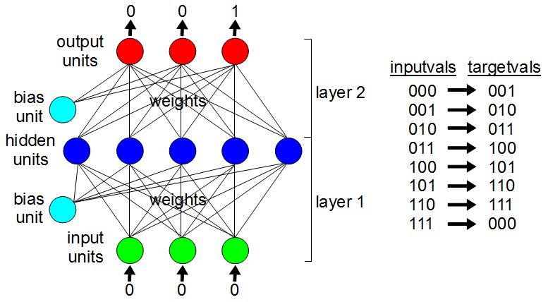
A simple neural network has some input units where the input goes. It also has hidden units, so-called because from a user’s perspective they’re literally hidden. And there are output units, from which we get the results. Off to the side are also bias units, which are there to help control the values emitted from the hidden and output units. Connecting all of these units are a bunch of weights, which are just numbers, each of which is associated with two units.
The way we instill intelligence into this neural network is to assign values to all those weights. That’s what training a neural network does, find suitable values for those weights. Once trained, in our example, we’ll set the input units to the binary digits 0, 0, and 0 respectively, TensorFlow will do stuff with everything in between, and the output units will magically contain the binary digits 0, 0, and 1 respectively. In case you missed that, it knew that the next number after binary 000 was 001. For 001, it should spit out 010, and so on up to 111, wherein it’ll spit out 000. Once those weights are set appropriately, it’ll know how to count.
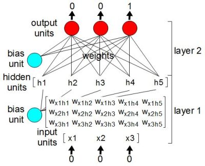
One step in “running” the neural network is to multiply the value of each weight by the value of its input unit, and then to store the result in the associated hidden unit.
We can redraw the units and weights as arrays, or what are called lists in Python. From a math standpoint, they’re matrices. We’ve redrawn only a portion of them in the diagram. Multiplying the input matrix with the weight matrix involves simple matrix multiplication resulting in the five element hidden matrix/list/array.
From Matrices to Tensors
In TensorFlow, those lists are called tensors. And the matrix multiplication step is called an operation, or op in programmer-speak, a term you’ll have to get used to if you plan on reading the TensorFlow documentation. Taking it further, the whole neural network is a collection of tensors and the ops that operate on them. Altogether they make up a graph.


Shown here are snapshots taken of TensorBoard, a tool for visualizing the graph as well as examining tensor values during and after training. The tensors are the lines, and written on the lines are the tensor’s dimensions. Connecting the tensors are all the ops, though some of the things you see can be double-clicked on in order to expand for more detail, as we’ve done for layer1 in the second snapshot.
At the very bottom is x, the name we’ve given for a placeholder op that allows us to provide values for the input tensor. The line going up and to the left from it is the input tensor. Continue following that line up and you’ll find the MatMul op, which does the matrix multiplication with that input tensor and the tensor which is the other line leading into the MatMul op. That tensor represents the weights.
All this was just to give you a feel for what a graph and its tensors and ops are, giving you a better idea of what we mean by TensorFlow being a “software library for numerical computation using data flow graphs”. But why we would want to create these graphs?
Why Create Graphs?
The API that’s currently stable is one for Python, an interpreted language. Neural networks are compute intensive and a large one could have thousands or even millions of weights. Computing by interpreting every step would take forever.
So we instead create a graph made up of tensors and ops, describing the layout of the neural network, all mathematical operations, and even initial values for variables. Only after we’ve created this graph do we then pass it to what TensorFlow calls a session. This is known as deferred execution. The session runs the graph using very efficient code. Not only that, but many of the operations, such as matrix multiplication, are ones that can be done on a supported GPU (Graphics Processing Unit) and the session will do that for you. Also, TensorFlow is built to be able to distribute the processing across multiple machines and/or GPUs. Giving it the complete graph allows it to do that.
Creating The Binary Counter Graph
And here’s the code for our binary counter neural network. You can find the full source code on this GitHub page. Note that there’s additional code in it for saving information for use with TensorBoard.
We’ll start with the code for creating the graph of tensors and ops.
import tensorflow as tf
sess = tf.InteractiveSession()

NUM_INPUTS = 3
NUM_HIDDEN = 5
NUM_OUTPUTS = 3
We first import the tensorflow module, create a session for use later, and, to make our code more understandable, we create a few variables containing the number of units in our network.
x = tf.placeholder(tf.float32, shape=[None, NUM_INPUTS], name='x')
y_ = tf.placeholder(tf.float32, shape=[None, NUM_OUTPUTS], name='y_')
Then we create placeholders for our input and output units. A placeholder is a TensorFlow op for things that we’ll provide values for later. x and y_ are now tensors in a new graph and each has a placeholder op associated with it.
You might wonder why we define the shapes as [None, NUM_INPUTS] and [None, NUM_OUTPUTS], two dimensional lists, and why None for the first dimension? In the overview of neural networks above it looks like we’ll give it one input at a time and train it to produce a given output. It’s more efficient though, if we give it multiple input/output pairs at a time, what’s called a batch. The first dimension is for the number of input/output pairs in each batch. We won’t know how many are in a batch until we actually give one later. And in fact, we’re using the same graph for training, testing, and for actual usage so the batch size won’t always be the same. So we use the Python placeholder object None for the size of the first dimension for now.
W_fc1 = tf.truncated_normal([NUM_INPUTS, NUM_HIDDEN], mean=0.5, stddev=0.707)
W_fc1 = tf.Variable(W_fc1, name='W_fc1')

b_fc1 = tf.truncated_normal([NUM_HIDDEN], mean=0.5, stddev=0.707)
b_fc1 = tf.Variable(b_fc1, name='b_fc1')

h_fc1 = tf.nn.relu(tf.matmul(x, W_fc1) + b_fc1)
That’s followed by creating layer one of the neural network graph: the weights W_fc1, the biases b_fc1, and the hidden units h_fc1. The “fc” is a convention meaning “fully connected”, since the weights connect every input unit to every hidden unit.
tf.truncated_normal results in a number of ops and tensors which will later assign normalized, random numbers to all the weights.
The Variable ops are given a value to do initialization with, random numbers in this case, and keep their data across multiple runs. They’re also handy for saving the neural network to a file, something you’ll want to do once it’s trained.
You can see where we’ll be doing the matrix multiplication using the matmul op. We also insert an add op which will add on the bias weights. The relu op performs what we call an activation function. The matrix multiplication and the addition are linear operations. There’s a very limited number of things a neural network can learn using just linear operations. The activation function provides some non-linearity. In the case of the relu activation function, it sets any values that are less than zero to zero, and all other values are left unchanged. Believe it or not, doing that opens up a whole other world of things that can be learned.
W_fc2 = tf.truncated_normal([NUM_HIDDEN, NUM_OUTPUTS], mean=0.5, stddev=0.707)
W_fc2 = tf.Variable(W_fc2, name='W_fc2')

b_fc2 = tf.truncated_normal([NUM_OUTPUTS], mean=0.5, stddev=0.707)
b_fc2 = tf.Variable(b_fc2, name='b_fc2')

y = tf.matmul(h_fc1, W_fc2) + b_fc2
The weights and biases for layer two are set up the same as for layer one but the output layer is different. We again will do a matrix multiplication, this time multiplying the weights and the hidden units, and then adding the bias weights. We’ve left the activation function for the next bit of code.
results = tf.sigmoid(y, name='results')

cross_entropy = tf.reduce_mean(
tf.nn.sigmoid_cross_entropy_with_logits(logits=y, labels=y_))
Sigmoid is another activation function, like the relu we encountered above, there to provide non-linearity. I used sigmoid here partly because the sigmoid equation results in values between 0 and 1, ideal for our binary counter example. I also used it because it’s good for outputs where more than one output unit can have a large value. In our case, to represent the binary number 111, all the output units can have large values. When doing image classification we’d want something quite different, we’d want just one output unit to fire with a large value. For example, we’d want the output unit representing giraffes to have a large value if an image contains a giraffe. Something like softmax would be a good choice for image classification.
On close inspection, it looks like there’s some duplication. We seem to be inserting sigmoid twice. We’re actually creating two different, parallel outputs here. The cross_entropy tensor will be used during training of the neutral network. The results tensor will be used when we run our trained neural network later for whatever purpose it’s created, for fun in our case. I don’t know if this is the best way of doing this, but it’s the way I came up with.
train_step = tf.train.RMSPropOptimizer(0.25, momentum=0.5).minimize(cross_entropy)
The last piece we add to our graph is the training. This is the op or ops that will adjust all the weights based on training data. Remember, we’re still just creating a graph here. The actual training will happen later when we run the graph.
There are a few optimizers to chose from. I chose tf.train.RMSPropOptimizer because, like the sigmoid, it works well for cases where all output values can be large. For classifying things as when doing image classification, tf.train.GradientDescentOptimizer might be better.
Training And Using The Binary Counter
Having created the graph, it’s time to do the training. Once it’s trained, we can then use it.
inputvals =  [[0, 0, 0], [0, 0, 1], [0, 1, 0], [0, 1, 1], [1, 0, 0], [1, 0, 1],
              [1, 1, 0], [1, 1, 1]]
targetvals = [[0, 0, 1], [0, 1, 0], [0, 1, 1], [1, 0, 0], [1, 0, 1], [1, 1, 0],
              [1, 1, 1], [0, 0, 0]]
First, we have some training data: inputvals and targetvals. inputvals contains the inputs, and for each one there’s a corresponding targetvals target value. For inputvals[0] we have [0, 0, 0], and the expected output is targetvals[0], which is [0, 0, 1], and so on.
if do_training == 1:
  sess.run(tf.global_variables_initializer())

  for i in range(10001):
    if i%100 == 0:
      train_error = cross_entropy.eval(feed_dict={x: inputvals, y_:targetvals})
      print("step %d, training error %g"%(i, train_error))
      if train_error < 0.0005:
        break

    sess.run(train_step, feed_dict={x: inputvals, y_: targetvals})

  if save_trained == 1:
    print("Saving neural network to %s.*"%(save_file))
    saver = tf.train.Saver()
    saver.save(sess, save_file)
do_training and save_trained can be hardcoded, and changed for each use, or can be set using command line arguments.
We first go through all those Variable ops and have them initialize their tensors.
Then, for up to 10001 times we run the graph from the bottom up to the train_step tensor, the last thing we added to our graph. We pass inputvals and targetvals to train_step‘s op or ops, which we’d added using RMSPropOptimizer. This is the step that adjusts all the weights such that the given inputs will result in something close to the corresponding target outputs. If the error between target outputs and actual outputs gets small enough sooner, then we break out of the loop.
If you have thousands of input/output pairs then you could give it a subset of them at a time, the batch we spoke of earlier. But here we have only eight, and so we give all of them each time.
If we want to, we can also save the network to a file. Once it’s trained well, we don’t need to train it again.
else: # if we're not training then we must be loading from file

  print("Loading neural network from %s"%(save_file))
  saver = tf.train.Saver()
  saver.restore(sess, save_file)
  # Note: the restore both loads and initializes the variables
If we’re not training it then we instead load the trained network from a file. The file contains only the values for the tensors that have Variable ops. It doesn’t contain the structure of the graph. So even when running an already trained graph, we still need the code to create the graph. There is a way to save and load graphs from files using MetaGraphs but we’re not doing that here.
print('\nCounting starting with: 0 0 0')
res = sess.run(results, feed_dict={x: [[0, 0, 0]]})
print('%g %g %g'%(res[0][0], res[0][1], res[0][2]))
for i in range(8):
res = sess.run(results, feed_dict={x: res})
print('%g %g %g'%(res[0][0], res[0][1], res[0][2]))
In either case we try it out. Notice that we’re running it from the bottom of the graph up to the results tensor we’d talked about above, the duplicate output we’d created especially for when making use of the trained network.
We give it 000, and hope that it returns something close to 001. We pass what was returned, back in and run it again. Altogether we run it 9 times, enough times to count from 000 to 111 and then back to 000 again.
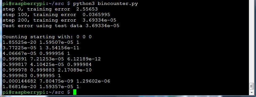
Here’s the output during successful training and subsequent counting. Notice that it trained within 200 steps through the loop. Very occasionally it does all 10001 steps without reducing the training error sufficiently, but once you’ve trained it successfully and saved it, that doesn’t matter.
The Next Step
As we said, the code for the binary counter neural network is on our github page. You can start with that, start from scratch, or use any of the many tutorials on the TensorFlow website. Getting it to do something with hardware is definitely my next step, taking inspiration from this robot that [Lukas Biewald] made recognize objects around his workshop.
What are you using, or planning to use TensorFlow for? Let us know in the comments below and maybe we’ll give it a try in a future article!


TensorFlow is integrating Keras as of the last versions to improve usability. If you’re going to work with NN’s, start with learning Keras.
You only need to bother with TensorFlow directly if you’re going to do research on new NN architectures or need to implement one that isn’t ported to Keras yet.
Don’t be so quick to dismiss TensorFlow, it’s perfectly usable directly. Much of what is available from Torch or Keras are convenience functions or predefined architectures.
That’s like saying “CUDA is perfectly usable directly, TensorFlow is just a layer with convenience functions or predefined architectures”.
Keras has been added to TensorFlow exactly because it’s a higher-level layer to make things simpler. This is an article about making NN’s in TensorFlow, there is nothing in this article that couldn’t be made using the Keras interface that wouldn’t be shorter and more readable using it.
There are plenty of reasons to learn TensorFlow, and to dig into it while using the Keras layer. But using it directly for a perceptron is not a good reason.
Keras is getting integrated, but it’s not there yet. I’m not going to jump into the contrib library just because it’s the new hotness. Use what works. Besides, if you understand NNs in TensorFlow, then you can always shift to Keras once everything settles down.
But yeah, by all means, if you wanna play around with MNIST and make a quick NN to check off an item on your bucket list or pad out a resume, then yeah, use a pre-built architecture in Keras. Can I also suggest the multilayer perceptron in scikit-learn? It’s got that easy interface and it’s super easy to install.
Re the contrib library, I’m the same way. On the TensorFlow website they say it’s subject to change so I stayed away.
Re Keras, I’m sure I’ve heard the name before, and just checked it out. I looks good, and can do all the code in the article, but if it’s not settled yet either then I’ll avoid it for now too.
That just personal preference.
There are already plenty of TensorFlow YouTube tutorials that are out of date and only six months old. Now that it’s stable I’ve dipped my toe in.
Keras isn’t fully integrated into TensorFlow, but the standalone Keras with TensorFlow and Theano backends has been working for quite a while now, is fully stable and has quite widespread use (not sure on the “market share” of Caffe/Torch/Keras/etc, people generally use whatever cross their path first)
@r4m0n Ah. Thanks for clarifying.
First, what’s a tensor:
https://www.youtube.com/watch?v=f5liqUk0ZTw
:o)
That was amazing. Thank you @RoGeorge
Thank you so much for posting this. I do computational chemistry for part of my research, and the anisotropy of NMR chemical shifts are calculated and described using “shielding tensors”, and while I haven’t really been using those results much this makes things make A LOT more sense from a mental visualization perspective.
This is amazing, exactly the sort of intro i was looking for. I would be looking in future to make hardware that could recognise and react to different types of sound.
https://www.extremetech.com/computing/247199-googles-dedicated-tensorflow-processor-tpu-makes-hash-intel-nvidia-inference-workloads
I’m looking forward to getting some hardware working with it too. Maybe some servos and sensors in a robot.
“What are you using, or planning to use TensorFlow for? Let us know in the comments below and maybe we’ll give it a try in a future article!”
Solving the problem of moderating trolls.
For this line: cross_entropy = tf.reduce_mean(tf.nn.sigmoid_cross_entropy_with_logits(logits=y, labels=y_))
I get the error:
Traceback (most recent call last):
File “”, line 1, in
TypeError: sigmoid_cross_entropy_with_logits() got an unexpected keyword argument ‘labels’
Might be an issue with your version of TensorFlow, as labels is a new argument for tf.nn.sigmoid_cross_entropy_with_logits
Here’s a relevant issue: https://github.com/carpedm20/DCGAN-tensorflow/issues/84
So does this mean I can speak to this neural network and discuss the meaning of life?
Can I make my own Jarvis?
Why not just ask a person? They’re a neural network with which you can discuss the mesning of life. They certainly would know more about it than a system that only has a handful of bits of input.
https://hackaday.io/project/20409-affordable-world-healthcare
Cool. And it looks like we can bring TFLearn into the mix.
“For inputvals[0][0] we have [0, 0, 0], and the expected output is targetvals[0][0], which is [0, 0, 1], and so on.”
Pretty sure you mean ‘inputvals[0]’ and ‘targetvals[0]’.
[0][0] would be 0 for both; [0][2] would be 0 and 1.
Yes, that’s what I meant. Good catch. Fixed. Thanks!
Thanks for this nice tutorial and code. Here is my binary-summation testing with Keras:
————————————
import numpy as np
import matplotlib.pyplot as plt
from keras import optimizers
from keras.models import Sequential
from keras.layers import Dense
from keras.callbacks import EarlyStopping
def getmodel():
model = Sequential()
model.add(Dense(4,name=”hidden”,input_dim=3, activation=’sigmoid’))
model.add(Dense(3,name=’output’, activation=’linear’))
sgd = optimizers.SGD(lr=0.5, decay=1e-6, momentum=0.9, nesterov=True)
model.compile(loss=’mean_squared_error’, optimizer=sgd)
return model
X=np.array(list(map(lambda x: list(map(int,list(bin(x)[2:].zfill(3)))),range(8))),dtype=bool)
Y=np.roll(X,-1,axis=0)
model=getmodel()
model.summary()
early_stopping = EarlyStopping(monitor=’loss’, patience=5)
model.fit(X,Y, epochs=30000,callbacks=[early_stopping])
# plotting
f, axarr = plt.subplots(1,3)
m=axarr[0].matshow(Y.astype(‘float’))
axarr[0].set_title(‘Correct responses’)
f.colorbar(m,ax=axarr[0])
m=axarr[1].matshow(model.predict(X))
axarr[1].set_title(‘Model’)
f.colorbar(m,ax=axarr[1])
m=axarr[2].matshow(np.round(model.predict(X)))
axarr[2].set_title(‘Model (rounded)’)
f.colorbar(m,ax=axarr[2])
Nice! I should install Keras and try it out. Thanks!
not working, can You send gist or gitlab example?
File “bincounter.py”, line 65, in
sess = tf.InteractiveSession()
AttributeError: module ‘tensorflow’ has no attribute ‘InteractiveSession’
sorry but not working