
Blurring is a commonly used visual effect when digitally editing photos and videos. One of the most common blurs used in these fields is the Gaussian blur. You may have used this tool thousands of times without ever giving it greater thought. After all, it does a nice job and does indeed make things blurrier.
Of course, we often like to dig deeper here at Hackaday, so here’s our crash course on what’s going on when you run a Gaussian blur operation.
It’s Math! It’s All Math.
Digital images are really just lots of numbers, so we can work with them mathematically. Each pixel that makes up a typical digital color image has three values- its intensity in red, green and blue. Of course, greyscale images consist of just a single value per pixel, representing its intensity on a scale from black to white, with greys in between.
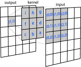
Regardless of the image, whether color or greyscale, the basic principle of a Gaussian blur remains the same. Each pixel in the image we wish to blur is considered independently, and its value changed depending on its own value, and those of its surroundings, based on a filter matrix called a kernel.
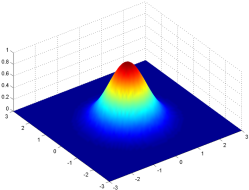
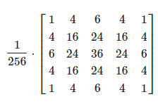
The kernel consists of a rectangular array of numbers that follow a Gaussian distribution, AKA a normal distribution, or a bell curve.
Our rectangular kernel consists of values that are higher in the middle and drop off towards the outer edges of the square array, like the height of a bell curve in two dimensions. The kernel corresponds to the number of pixels we consider when blurring each individual pixel. Larger kernels spread the blur around a wider region, as each pixel is modified by more of its surrounding pixels.
For each pixel to be subject to the blur operation, a rectangular section equal to the size of the kernel is taken around the pixel of interest itself. These surrounding pixel values are used to calculate a weighted average for the original pixel’s new value based on the Gaussian distribution in the kernel itself.
Thanks to the distribution, the central pixel’s original value has the highest weight, so it doesn’t obliterate the image entirely. Immediately neighboring pixels having the next highest influence on the new pixel, and so on. This local averaging smoothes out the pixel values, and that’s the blur.
Edge cases are straightforward too. Where an edge pixel is sampled, the otherwise non-existent surrounding pixels are either given the same value of their nearest neighbor, or given a value matching up with their mirror opposite pixel in the sampled area.
The same calculation is run for each pixel in the original image to be blurred, with the final output image made up of the pixel values calculated through the process. For grayscale images, it’s that simple. Color images can be done the same way, with the blur calculated separately for the red, green, and blue values of each pixel. Alternatively, you can specify the pixel values in some other color space and smooth them there.
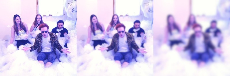
Here we see an original image, and a version filtered with a Gaussian blur of kernel size three and kernel size ten. Note the increased blur as the kernel size increases. More pixels incorporated in the averaging results in more smoothing.
Of course, larger images require more calculations to deal with the greater number of pixels, and larger kernel sizes sample more surrounding pixels for each pixel of interest, and can thus take much longer to calculate. However, on modern computers, even blurring high-resolution images with huge kernel sizes can be done in the blink of an eye. Typically, however, it’s uncommon to use a kernel size larger than around 50 or so as things are usually already pretty blurry by that point.
The Gaussian blur is a great example of simple mathematics put to a powerful use in image processing. Now you know how it works on a fundamental level!


You can also use kernel’s to highlight features in an image like detecting edges by suppressing everything that is not high contrast (ref: https://en.wikipedia.org/wiki/Kernel_(image_processing) )
I used a Gaussian blur for my etch a selfie project (https://hackaday.com/2019/07/30/etch-a-selfie/)
There two Gaussian blurs are subtracted and this makes it possible to convert Images into nice black-and-white images.
(ref: XDog https://users.cs.northwestern.edu/~sco590/winnemoeller-cag2012.pdf)
That’s a great paper. I’ve been using a hillbilly version of that algorithm for my hanging plotter project but this one is significantly nicer! How did you stumble upon it?
I don’t remember … It was years ago where I implemented an BW filter for laser.im-pro.at ….
Also the classic Sharpen filter is a RREF-style reversal of a gaussian blur kernel. Meanwhile Unsharp Mask is a gaussian blur applied in negative which is why it’s easier to parametrize: there’s no solving step.
now how about inverting an applied gaussian blur to recover the prior image.
Ah, the fun worlds of deconvolution, and blind deconvolution.
And if you apply the same blur sequentially? Are two 3×3 blurs the same as a single 5×5?
I guess I should do some math…
Yep, doing the math helps here, to some degree:
the convolution of a Gaussian with a Gaussian is still a Gaussian (without that, there wouldn’t be the central limit theorem, i.e. the reason why sums of independent identically distributed random variables add up to Gaussian distribution for large numbers of summands). So, yes, if we take a Gaussian with some sigma² and convolve it with itself, we get a new Gaussian with twice the sigma² (Variance).
This means that if we decided the original discrete 3×3 kernel was “large” enough to cover the “interesting parts of the Gaussian because the stuff that was “cut off” from the (infinitely extending) Gaussian function was small enough for our tastes to not matter.
(I’m ***very*** much at odds with the article: “larger kernels spread further”: No; you can put the same 3×3 in a 11×11 matrix and fill in with the smaller values from the actual Gaussian function. What the author means is that a higher-variance Gaussian spreads further.)
But 5 is not at least twice 3… so, you’d get a worse approximation to an actual Gaussian filter with this finite kernel.
However 5×5 is indeed the size you get when you, in the discrete domain, convolve two 3×3 kernels. So, by doing it that way, you get a different Gaussian kernel, but it’s a worse approximation to the Gaussian of twice the variance of the Gaussian in the 3×3 kernel.
Also the Gaussian is separable, so you can do the 2D blur by doing a 1D horizontally and then vertically.
Is it just me that’s bothered by the logo in the post header *not* being the result of the sharp hackaday logo being filtered with a symmetric kernel,i.e. especially *not* with a Gaussian? That blur isn’t symmetrical at all!
Nope, not just you. That kinda jumped out at me as well.
Honestly, I like when HaD does such articles!
I must still voice my disagreement on a few things: the first two are fundamental, the third I think is a bit of an overgeneralization but not a fundamentally wrong statement; my apologies.
> The kernel consists of a rectangular array of numbers that follow a Gaussian distribution,
Please be careful with the terminology here; what you write will mislead readers :(
These numbers don’t follow a Gaussian distribution. They are deterministic; they are samples taken from the *Gaussian function*, which happens to be the probability density of the Gaussian distribution.
> Larger kernels spread the blur around a wider region,
This is wrong – the size of the kernel doesn’t define the spread, just the number of pixels taken into account.
The spread is defined by the variance of the Gaussian function that gets sampled for the kernel. You can have a very narrow blur “spread” in a large filter, if you need the accuracy, or a very wide (=high variance) blur in a small filter.
The question is really just how much of the actual continuous function you cut off when you decide on your filter size.
But these are two different properties of the filter, and you’re conflating them!
> as each pixel is modified by more of its surrounding pixels.
That’s right – a larger Kernel takes more pixels into account.
> Edge cases are straightforward too. Where an edge pixel is sampled, the otherwise non-existent surrounding pixels are either given the same value of their nearest neighbor, or given a value matching up with their mirror opposite pixel in the sampled area.
These are **two** options, but they are not necessarily the right ones for any particular application. In fact, that choice can become very awkward for the pixels that are not at the very image border – the actual border pixel get their “weight” increased very much, so that their values overshadow that of their neighbors.
So, not a great generalization to make!
Now for a math routine to put shake and jiggle into stable video and stills for enhanced viewing.
Oh god, don’t give them ideas! We already have fake film lines and blemishes, and fake artefacts and glitches. Overuse of those is bad enough.
I would question the large kernels taking significant processing time. Applying the blur is a convolution and almost any sensible algorithm will actually compute this as a multiplication in Fourier space. Take your kernel and image, FFT both, multiple them together and then do in the inverse FFT. Almost certainly massively faster than a direct real space convolution where you generate a new image, multiple every pixel by the kernel and sum the the relevant pixels into the results image.
ROFL. Nope. Gaussian kernels are separable, and can use the central limit theorem, plus some linear and constant time algorithms, to do the work much more quickly than you could do a 2D FFT (much less the multiply and reverse FFT). Plus the separability makes the operation much more cache friendly than an FFT. (see also: bicubic and sinc based resampling kernels)
If you are doing a convolution that isn’t separable, then an FFT (or other frequency space transform) might be a good idea. But please talk to algorithms and performance experts first, and measure, measure, measure.
FFT is faster for large data.
https://ccrma.stanford.edu/~jos/ReviewFourier/FFT_Convolution_vs_Direct.html
The source you linked to only considers theoretical number of operations. In practice, memory access order and caches are far more important. The crossover point where FFT-based convolution is faster than separable convolution will only happen for much larger inputs.
Yeah, that completely ignores better algorithms and cache effects. It’s using the number of operations for a direct convolution – not separable, not box filters (certainly not the constant time algorithms for box filters).
Next time, you probably should consult with someone who actually knows algorithms and performance.
These people at Analog Devices are idiots. Shouldn’t consult them at all.
“”This chapter presents two important DSP techniques, the overlap-add method, and FFT
convolution. The overlap-add method is used to break long signals into smaller segments for
easier processing. FFT convolution uses the overlap-add method together with the Fast Fourier
Transform, allowing signals to be convolved by multiplying their frequency spectra. For filter
kernels longer than about 64 points, FFT convolution is faster than standard convolution, while
producing exactly the same result. “”
https://www.analog.com/media/en/technical-documentation/dsp-book/dsp_book_Ch18.pdf
Mr Algorithm guru would you be so kind as to point me to where I can gain understanding about this from the REAL experts?
Yes sparky, you are in way over your head. FFTs are good in some places, and not in many others. In real world image processing, an FFT for gaussian blur would be among the slowest algorithms (only exceeded by brute force convolution). You are confusing theory (written by people who don’t know the practice and who are talking entirely in generalities) with actual practice. I’m talking about actual code in major applications that has been highly optimized, measured, copied by other applications, and hits the limits for throughput on a variety of architectures and inputs (image size, kernel size, etc.).
How can you gain experience? Listen to the experts and stop trying to claim you know more than they do by quoting other people who know even less.
Here’s a hint: click on the link in my name above.
Ok smartie Chris. You win. All i did was google fft vs convolution and the first 63455 articles all went with fft as faster once past a very minimal kernel size. I looked for something agreeing with you but couldn’t find it. One thing i have always noticed is that when someone makes the boneheaded claim about the difference between theory and practice they don’t actually know the theory. What they have in brain is a conglomeration of anecdotes that support their view.
Again, sparky, you are in way over your head.
You thought you could “one up” the experts by looking things up on Google. But you got the theory (and ignored all the warning signs that it was just theory), with zero practice and zero experience.
Again, you probably should click on the link in my name here to learn who it is that you are addressing. Yes, I know the theory, and I lecture on it a few times a year at the larger universities here in the SF Bay Area. I also spent many years on the practice: measuring everything, improving the algorithms until they were limited by the speed of RAM instead of the CPU, squeezing out a bit more performance with significant cache optimization, then re-optimizing for each new major chip architecture. There is a reason why the chip and motherboard makers consult with me about their latest designs and how their changes will affect real world throughput…
Next time, try asking questions instead of claiming the experts are wrong based on your 5 seconds of Google “research”.
Hallo Chris,
I really appreciate your input to this topic. I’m now myself working in a research institute and my experience is not really good. We have an high incentive to write publications and there the quality is often not optimal. Furthermore when doing research I takes a lot of effort to filter out bad papers and find the practical problems.
I hob if somebody searches about FFT for convolution this will show up to save them a lot of time to go throw with the implementation and find in the end that it will not be faster for real applications.
Thanks Chris!
@sparky here is one link about chis you should open : http://www.photoshophalloffame.com/chris-cox
The article would be greatly improved if the actual formula for pixel weighting was provided.
Yeah, it is lacking a bit in detail.
See https://en.wikipedia.org/wiki/Gaussian_filter
you guys are gaussian blurring and im still reticulating splines :(
If you have any interest in stitching images together (to make a panorama) then it helps to know about Gaussian blur.
Blurring to different kernel sizes, then subtracting (Difference of Gaussians), is one of the steps in keypoint detection algorithms like SIFT and SURF.
https://en.wikipedia.org/wiki/Image_stitching#Keypoint_detection