You probably have at least a nodding familiarity with the Fourier transform, a mathematical process for transforming a time-domain signal into a frequency domain signal. In particular, for computers, we don’t really have a nice equation so we use the discrete version of the transform which takes a series of measurements at regular intervals. If you need to understand the entire frequency spectrum of a signal or you want to filter portions of the signal, this is definitely the tool for the job. However, sometimes it is more than you need.
For example, consider tuning a guitar string. You only need to know if one frequency is present or if it isn’t. If you are decoding TouchTones, you only need to know if two of eight frequencies are present. You don’t care about anything else.
A Fourier transform can do either of those jobs. But if you go that route you are going to do a lot of math to compute things you don’t care about just so you can pick out the one or two pieces you do care about. That’s the idea behind the Goertzel. It is essentially a fast Fourier transform algorithm stripped down to compute just one frequency band of interest. The math is much easier and you can usually implement it faster and smaller than a full transform, even on small CPUs.
Fourier in Review
Just to review, a typical system that uses a Fourier transform will read a number of samples at some clock frequency using an analog to digital converter. For example, you might read 1024 samples at 1 MHz. Each sample will be 1 microsecond after the previous sample, and you’ll get just over a millisecond’s worth of data.
The transform will also produce 1024 results, often known as buckets. Each bucket will represent 1/1024 of the 1 MHz. Because of the Nyquist limit, the top half of the results are not very useful, so realistically, the first 512 buckets will represent 0 Hz to 500 kHz.
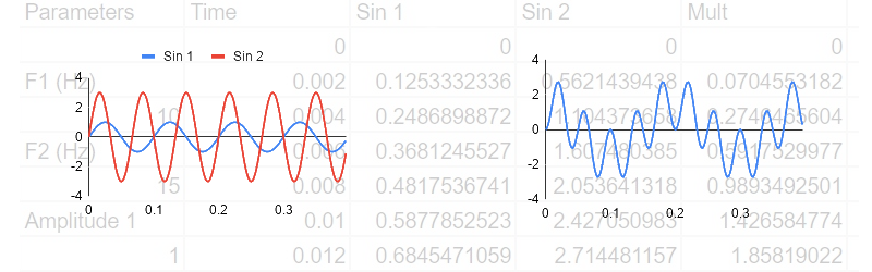
Here’s a spreadsheet (after all, this is the DSP Spreadsheet series of articles) that uses the XLMiner Analysis Addon to do Fourier transforms. The sample frequency is 1024Hz so each bucket (column G) is worth 1 Hz. Column B generates two sine waves together at 100 Hz and 20 Hz. We talked about generating signals like this last year.
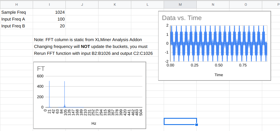
The FFT data in column C are complex numbers and they do not update live. You have to use the XLMiner add on to recompute it if you change frequencies. The magnitude of the numbers appear in column F and you’ll see that the buckets that correspond to the two input frequencies will be much higher than the other buckets.
One Bucket of Many
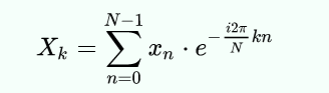
If our goal was to find out if the signal contained the 100 Hz signal, we could just compute cell F102, if we knew how. That’s exactly what the Goertzel does. Here’s the actual formula for each bucket in a discrete Fourier transform (courtesy of Wikipedia):
If you apply Euler’s formula you get:
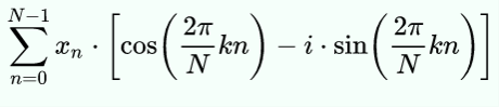
Mathematically, N is the block size, k is the bucket number of interest, xn is the nth sample. Since n varies from 0 to N-1, you can see this expression uses all of the data to compute each bucket’s value.
The trick, then, is to find the minimum number of steps we need to compute just one bucket. Keep in mind that for a full transform, you have to do this math for each bucket. Here we only need to do it for one. However, you do have to sum up everything.
Cut to the Chase
If you do a bit of manipulation, you can reduce it to the following steps:
- Precompute the frequency ratio in radians which is 2Πk/N
- Compute the cosine of the value you found in step 1 (call this C); also compute the sine (call this S)
- For each bucket in sequence, take the value of the previous bucket (P) and the bucket before that (R) and compute bucket=2*C*P-R and then add the current input value
- Now the last bucket will be set up to nearly give you the value for the kth bucket. To find the real part, multiply the final bucket by C and subtract P. For the imaginary part, multiply S times the final bucket value
- Now you want to find the magnitude of the complex number formed by the real and imaginary parts. That’s easy to do if you convert to polar notation (find the hypotenuse of the triangle formed by the real and imaginary part).
Of course, there’s a spreadsheet for this, too. With the limitations of a spreadsheet, it does a lot of extra calculations, so to make up for it, column D hides all the rows that don’t matter. In a real program you would simply not do those calculations (columns E-G) except for the last time through the loop (that is, on each row). You need a few samples to prime the pump, so the first two rows are grayed out.
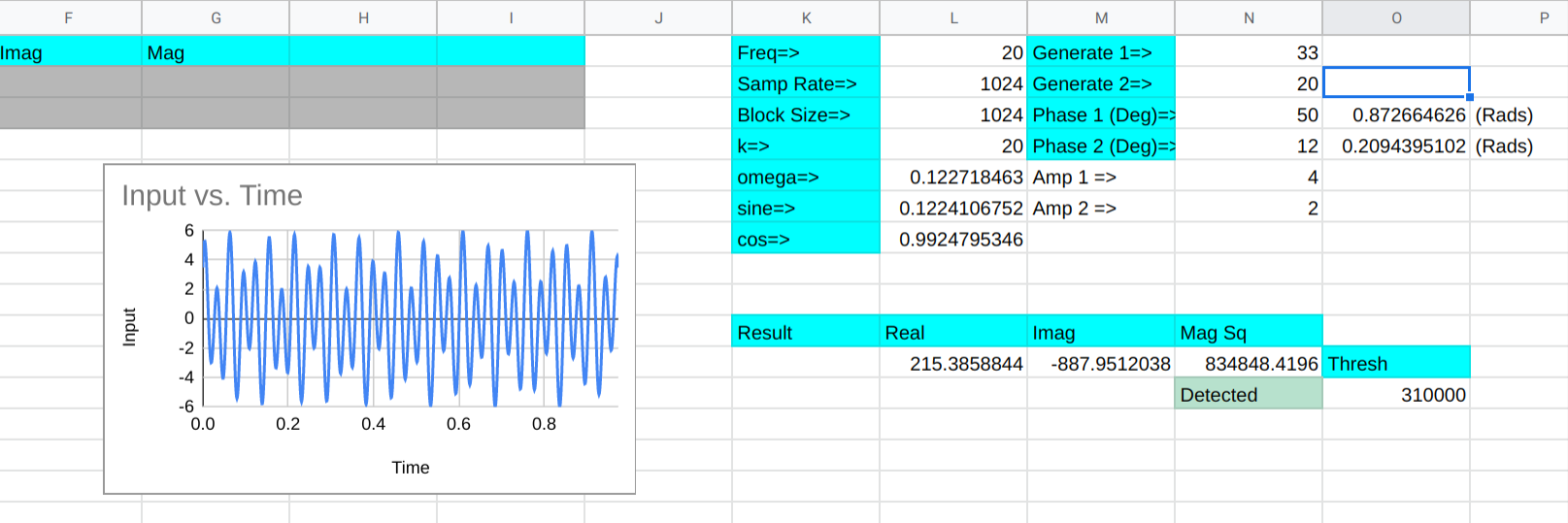
There are other optimizations you’d make, too. For example, the cosine term is doubled each time through the loop but not on the final calculation. In a real program, you’d do that calculation once, but for a small spreadsheet, there’s not much difference.
Column B is the input data, of course. Column C is the running total of the buckets. Columns E-G on the last row represents the final computations to get the bucket k’s complex result. The real place to look for the results in around L11. That part of row 11 picks up the one visible part of columns E-G and also squares the magnitude since we are looking for power. There’s also a threshold and a cell that tells you if the frequency (at L1) is present or not.
Try changing the generated frequencies and you’ll see that it does a good job of detecting frequencies near 20 Hz. You can adjust the threshold to get a tighter or broader response, but the difference between 20 Hz and 19 or 21 Hz is pretty marked.
Real Code
Since a spreadsheet doesn’t really give you a feel for how you’d really do this in a conventional programming language here is some pseudo-code:
omega_r = cos(2.0*pi*k/N);
omega_r2=2*omega_r;
omega_i = sin(2.0*pi*k/N);

P = 0.0;
S = 0.0;
for (n=0; n<N; ++n)
{
   y = x(n) + omega_r2*P -S;
   S = P;
   P = y;
}
realy = omega_r*P - S; // note that hear P=last result and S is the one before
imagy=omega_i*P;
magy=abs(complex(realy,imagy));  // mag=sqrt(r^2+i^2);
Since you can precompute everything outside of the loop, this is pretty easy to formulate in even a simple processor. You could even skip the square root if you are only making comparisons and want to square the result anyway.
Tradeoffs
Don’t forget, everything is a tradeoff. The sampling rate and the number of samples determine how long it takes to read each sample and also how broad the frequency range for the bucket is. If you are having to probe for lots of frequencies, you might be better off with a well-implemented Fourier transform library.
There are other ways to optimize both algorithms. For example, you can limit the amount of data you process by selecting the right sample rate and block size. Or, instead of using a Fourier transform, consider a Hartley transform which doesn’t use complex numbers.
In Practice
I doubt very seriously anyone needs to do this kind of logic in a spreadsheet. But like the other DSP spreadsheet models, it is very easy to examine and experiment with the algorithm laid out this way. Developing intuition about algorithms is at least as important as the rote recollection of them — maybe it is even more important.
The Goertzel is an easy way to sidestep a more complicated algorithm for many common cases. It is a tool you should have in your box of tricks.


Hideously complicated spreadsheets! Me like.
I’m more curious how to do that in e.g. small MCU. Especially without floats, etc. Sure, it’s nice to throw full blown abstract formulaes, full of floating points, sin/cos computing and somesuch. And every textbook does so, etc. What’s hard however is understanding how to do it FAST using MODEST resources, like e.g. MCU that lacks DSP. Old devices did e.g. DTMF recognition in software, using shy 6502 or Z80 – and were damn good at detecting their signals. That’s how you learn firmware is coded by real pro. But, seems these days it turned into kind of black magic. So you get textbook examples – but not really told how to do it efficient way using limited resources on cheap MCU. At most you get huge libs that solve all kinds of humankind problems, and things beyond that. However they are still to huge to grasp their inner working. Or heavily optimized for dozen and half of platforms to extent you can’t really grasp code flow at all.
DTMF Encoding & Decoding, An application of the Goertzel Algorithm:
http://stevenmerrifield.com/papers/hons_thesis.pdf
I used the Goertzel algorithm on a PIC 16Fxxx back in 2000 for decoding DTMF tones. All code was in PIX assembly language.
If you choose k/N “wisely” you can make omega_r be something like 1 or 0.5 or even 0.25.
The calculations then don’t need the multiply.
And using a coarse approximation to the square root of the sum of the squares can improve the speed. At the expense of accuracy though. But abs(smaller)/2+abs(larger) is typically within about 10%. One Newton iteration can get you to 1%, but you need a couple of multiplies. Still faster than a square root.
Assembly versions of square root aren’t much more difficult or slower than division. I always include this primitive in my Forth systems.
All this helps if your silicon is closer to a 555 than a floating point M4.
I am confused by the “Fourier in Review” part.
Sampling at 1MHz and then not being able to tell something about the frequencies > 500Hz?
You’re off by several orders of magnitude there. First you probably should be talking about buckets for 1 to 500kHz. And then the reasoning with “Nyquist” is still quite off:
We’re talking about the Discrete Fourier Transformation here, and since we’re feeding real input values (as opposed to complex values) into the algorithm the output will be symmetrical. That is a mathematical property of the DFT. There might be a connection between Nyquist and the DFT, but your reasoning feels way too much like handwaving here.
So are you seriously not able to figure out that this was a typo, or are you just being an ass? I mean, not that that’s a bad thing..
I think he DID recognize it as a typo, but there was ALSO a secondary concern.
But the secondary concern goes away when you realize the sampling frequency should have been 1 kHz. In any case, when you do the DFT, with 1 kHz sampling, you don’t GET any buckets above 500 Hz.
If you do a DFT with 1024 samples you get a result with 1024 Buckets. If you put in real values (as for e.g. audio samples) you might know that the upper half of the buckets gets the same values as the lower half (in a symmetrical fashion) and you may choose to not calculate them. But as I said: This is a property of the DFT for a specific subset of input values. Using “Nyquist” as an explanation to explain away the upper half of the buckets is IMHO quite wrong, since it basically implies that the higher buckets are for the frequencies >512Hz, which is just not the case.
If you know that the upper buckets contain the same values as the lower buckets, why would you even calculate them? This is absurd. In a Fourier transform, you provide half as many buckets as you have samples, but you have two values for each bucket (for real and imaginary parts, as you say), but you don’t go past 1/2 the sampling rate with these buckets.
The generic DFT allows for complex-valued input and has complex-valued output. The number of input and output coefficients is the same and of course it no longer behaves symetrically when you have complex input values.
*if* you have input values with no imaginary part, i.e. real values like e.g. audio samples. *then* you’re of course better off to not at all calculate the upper half of the outputs. And I am not disputing that it makes sense. Of course it does.
But claiming that “Because of the Nyquist limit, the top half of the results are not very useful” is just the wrong argument here.
Yeah we dropped a K somewhere in there.
Mmm, K
So what you are saying is, the Goertzel Algorithm is to the Fourier Transform, as a car radio with a few presets is to a spectrum analyzer.
I loved it when I was introduced to the Fourier transform long ago, and recognized all of the components of a zero IF radio receiver in it.
I have to admit, though, that to this day, my brain just screeches to a halt when it sees the collection of Greek letters in the Fourier Transform that just represents a sine wave, e^(-i). Don’t know why, maybe because i STILL don’t believe that a sine function is just an imaginary exponential. I am SO much happier with the Euler expansion of it into its real and imaginary parts. I guess because it says “sin” and “cos” in it instead of that exponential nonsense. You can explain it to my until you’re blue in the face, but I CAN’T look at e^(-i) and see a periodic function.
Have you watched Michael Ossman’s SDR tutorial series on youtube where he draws on the screen (for some reason they’re under someone else’s username)? The series is super-informative regarding complex exponentials. I believe Rick Lyons has also made some introductory papers available that are very good.
Oh, I’ve seen the explanations; they were very clear about this in my engineering program, and I can work in time or frequency domain with no problem. It’s just counterintuitive to the point of being useless, to refer to exponential functions as being periodic. It’s like telling me, over and over, that the sky is pink, and explaining it with detailed proofs and citations. And then I look at the sky and it’s still blue. It’s not that I don’t understand the math. It’s not that I can’t use the math. It’s that it fails the smell test and offends me greatly. But I’ll look that up, just to hear someone else’s wrong, wrong, wrong explanation. Thanks in advance.
There’s a good complex analysis lecture video. Google “downfall complex analysis”.
Actually, [e], I took [Henry]’s advice, and just finished watching Michael Ossman’s video series, part 6 (https://www.youtube.com/watch?v=37N0ra1CnnI&list=PL75kaTo_bJqmw0wJYw3Jw5_4MWBd-32IG&index=6), which is specifically all about complex numbers. ALL about them. (Thank you very much, Henry, for seeing right through my “I’ve heard it all before” bluster.) Ossman actually DOES have an explanation I hadn’t heard before, which freaking DOES make sense, which I expect I will fully assimilate once I watch it again tomorrow.
Anyway, [e], I appreciate your tip, but did you actually Google “downfall complex analysis” before recommending that? Most of the links were about societal collapse, and the first recommendation was, I kid you not, an article about Hitler. Which I don’t think is what we have been discussing. Please let me know if I misunderstood. Anyway, if there was a particular article you think would be helpful to myself and others, I’m sure we would all appreciate a link.
It is all about the Argand Diagram, Euler’s identity, and Euler’s formula for cos(u) + isin(u) and what happens when you multiply complex numbers. Virtually everyone regrets ever calling complex numbers the “real” and “imaginary” parts. It should be a vector with its own version of a product in modern education.
Probably because many people don’t see i and -i as rotations when they are used as exponents. Once you do, the whole Cartesian system makes sense.
The Goertzel algorithm is my go to for modulated detection tasks! especially with arm cmsis you can create it by using the iir biquad structure.
OK, I admit tldr at the moment, but are we talking about an Optimal Filter?
Goertzel algorithm is nice in also that you can analyze signals with a sliding window. It is possible to combine exponential sliding average directly in the structure, so that you don’t need to divide the incoming signal into blocks for computation like with FFT.
It is entirely possible to do a continuous Fourier transform as well, and applications of the Fourier transform almost always use windowing functions to reduce artifacts caused by the abrupt start and end of a signal. I will admit that I’d never heard of the Goertzel algorithm before, but it appears to be identical to the Fourier transfom in application, with the exception of the loop range. That is, it looks to me like the Goertzel algorithm is just the inner loop of the Fourier transform.
Goertzel is indeed just one bin of a discrete Fourier transform. If storage isn’t an issue and you’re going to be computing the same bin multiple times, it’s computationally faster in most modern languages to precompute one row of the DFT matrix and do a vector multiplication of that with the data column vector. It will give a slightly better answer than a Goertzel computation given that the multiplications are floating point and not “real.” If storage is an issue or if you are only doing one data set at a given bin, the Goertzel may be better. It permits precomputing only a couple of values and has very little internal storage, as it is a feedback algorithm.
Yes, that’s what I meant, but didn’t have the skills to describe properly. It’s still not exactly trivial because if you want to do any windowing function (and you usually DO), you can’t just subtract the oldest samples as you delete them and add the new ones. Which I think you also imply. But in any case, computing individual buckets is less expensive when that’s all you really need.
Spreadsheets… Use Octave
function freq_mag= EasyFFT(data,fs)
G = fft(data);
G = fftshift(G);
[cl rw] = size(G);
if rw > cl
G = G’; % sent in row form
endif
NumSamples = max(size(G));
df = fs / NumSamples;
f = ([ -(ceil((NumSamples-1)/2):-1:1), 0, (1:floor((NumSamples-1)/2)) ] * df)’;
ind = find(f==0);
freq_mag = [f(ind:end) abs(G(ind:end))];
endfunction
As it’s part of Office, I’ve used Excel for years. I’m reasonably familiar with the basics as a result, and I suspect many others fit the same description. For example, I know how to select a bunch of cells, and produce a graph.
Octave is, I believe, like Matlab. I haven’t used either, so I can’t be sure. The way you have a bunch of code reminds me of Python – but I’ve no idea how to graph any output.
Octave is probably more powerful, but without that familiarity it’s doomed when explaining basic concepts. Unless, of course, you want to write a series of articles for Hackaday? You could show how to do things in Excel, then repeat them in Octave. that would make an interesting series.
I use the Goertzel algorithm in my macOS SDR app to determine the CTCCS tones in radio signals: https://github.com/getoffmyhack/waveSDR
Here is the algorithm in Swift: https://github.com/getoffmyhack/waveSDR/blob/master/waveSDR/SDR/DSP/ToneDecoderBlock.swift
DTMF will be added at some point.
Also, I am no expert on DSP, this is just what worked for me after doing the research.