Last time I talked about how I took the open source Verifla logic analyzer and modified it to have some extra features. As promised, this time I want to show it in action, so you can incorporate it into your own designs. The original code didn’t actually capture your data. Instead, it created a Verilog simulation that would produce identical outputs to your FPGA. If you were trying to do some black box simulation, that probably makes sense. I just wanted to view data, so I created a simple C program that generates a VCD file you can read with common tools like gtkwave. It is all on GitHub along with the original files, even though some of those are not updated to match the new code (notably, the PDF document and the examples).

If you have enough pins, of course, you can use an external logic analyzer. If you have enough free space on the FPGA, you could put something like SUMP or SUMP2 in your design which would be very flexible. However, since these analyzers are made to be configurable from the host computer, they probably have a lot of circuitry that will compete with yours for FPGA space. You configure Verifla at compile time which is not as convenient but lets it have a smaller footprint.

Setup

I changed the way the original code worked for configuration quite a bit. In particular, I moved the config_verifla.v file to the project directory and out of the library. Then I consolidated several items in that file and reordered them. Here’s a portion of an example file (you can read the full file on GitHub):

// ********* TIMING and COMMUNICATONS
parameter CLOCK_FREQUENCY = 12_000_000;
// If CLOCK_FREQUENCY < 50 MHz then BAUDRATE must be < 115200 bps (for example 9600).
parameter BAUDRATE = 9600;
// The Baud Counter Size must have enough bits or more to hold this constant
parameter T2_div_T1_div_2 = CLOCK_FREQUENCY / (BAUDRATE * 16 * 2);
// Assert: BAUD_COUNTER_SIZE >= log2(T2_div_T1_div_2) bits
parameter BAUD_COUNTER_SIZE = 15;

// ********* Data Setup
// Number of data inputs (must be a multiple of 8)
parameter LA_DATA_INPUT_WORDLEN_BITS=16;

// ******** Trigger
// Your data & LA_TRIGGER_MASK must equal LA_TRIGGER_VALUE to start a complete capture
parameter LA_TRIGGER_VALUE=16'h0002, LA_TRIGGER_MASK=16'h0003;

// To help store more data, the LA counts how many samples are identical
// The next parameter is the size of the repeat count. Must be a multiple of 8 bits
// If the count overflows you just get another sample that starts counting again.
parameter LA_IDENTICAL_SAMPLES_BITS=16;

// ******** Memory Setup
parameter LA_MEM_ADDRESS_BITS=10; 
parameter LA_MEM_FIRST_ADDR=0,
          LA_MEM_LAST_ADDR=1023;
parameter LA_TRIGGER_MATCH_MEM_ADDR=513;
parameter LA_MAX_SAMPLES_AFTER_TRIGGER_BITS=24; 
parameter LA_MAX_SAMPLES_AFTER_TRIGGER=100000;

// Set this to 1 if you want to fill the buffer with a marker value
parameter LA_MEM_CLEAN_BEFORE_RUN=1;
parameter LA_MEM_EMPTY_SLOT=8'hEE;

// ********** Below this you shouldn't have to change anything

I removed most of the comments to keep it short, but you can find detailed comments in the GitHub copy. Obviously, you need to set the clock speed and baud rate. You also need to tell the analyzer how many samples to grab at once. This must be a multiple of 8 and, in this case, I used 16. Along with the sample there is a repeat count and that’s the size given by LA_IDENTICAL_SAMPLES_BITS. The larger the count, the more repeating data values you can compress, but the more waste there is when data doesn’t stay the same.

Of course, this file only sets up parameters. You still have to connect the signals you want. To do that, you have to make a simple change to your code.

Acquiring Data

Somewhere in your top module, you need something like this:

top_of_verifla verifla(.clk(clk),.cqual(1'b1),.rst_l(lareset), .sys_run(1'b0),
.data_in({ctimer,6'b0,state}),
.uart_XMIT_dataH(RS232_Tx),
.uart_REC_dataH(RS232_Rx)
);

The parameters are simple:

• clk – The system clock
• cqual – Clock qualifier; set low to ignore a clock cycle
• rst_l – Active low reset
• sys_run – Set high to cause the analyzer to run (see text below)
• uart_XMIT_dataH – Serial transmit pin
• uart_REC_dataH – Serial receive pin
• data_in – The data you want to capture. You can use brackets to join together as many bits as you specified in the configuration
• trigqual (not used here) – Set high to enable triggering
• exttrig (not used here) – Set high to trigger regardless of trigqual
• armed (not used here) – An output that goes high when the system is armed and waiting for a trigger
• triggered (not used here) – An output that goes high when the system is triggered

The sys_run input is a left over from the original code. If you set it to one, the system will pretty much be armed constantly. If your trigger occurs frequently, this will make it difficult for the host computer software to find the start of the data and you’ll probably get poor results.

I took advantage of the fact that many tools will allow you to use System Verilog features and provided defaults for parameters you often don’t need to set explicitly. For example, cqual is set to 1 and sys_run is set to 0. Unfortunately, some tools won’t do that. The version fo the Intel/Altera tools I use, for example, won’t recognize that even if you check the System Verilog box in the settings. To work around that, there is another version of the module in to_of_verifla_nodef.v you can use. If you do, though, you must set all the input parameters yourself.

In normal operation, the module sits idle (assuming sys_run is low) until it received a command from the PC via the serial port. There are only two commands. A binary 0 resets the unit and a 1 causes it to arm.

As I mentioned, the Java program from the original does this, reads the data, and builds a Verilog model that can create the output waveform. I wrote a C program that does basically the same thing but builds a VCD file instead. The lower-case command line parameters must match the settings in the Verilog configuration file. Here’s the help text:

Usage: la2vcd [-B] [-W] [-F frequency] [-T timescale] -b baud, -t trigger_pos -c cap_width, -r repeat_width, -n samples -o vcd_file port_name
You need all the lower case options, although baud will default to 9600
-B output only bytes of capture
-W output only words (default is both bytes and words)
-F sets frequency in MHz (e.g., -F 250).
Or you can set the timescale (e.g, -T 1ns) with -T. 
Note the timescale should be twice the clock frequency. 
Default to 1nS and you do your own math.

The other parameters (-B, -W, -F, and -T) are optional. A typical command line that would match the above configuration would be:

la2vcd -B -F 12 -t 513 -c 2 -r 2 -n 1024 -o test.vcd /dev/ttyUSB0

Note the width parameters are in bytes, so a 16 in the configuration will be a 2 on the command line. The command will wait for a trigger and read the data, writing it to test.vcd. You can open that file using any VCD viewer, such as gtkwave.

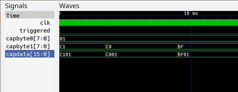
Reading the Data — gtkwave Tricks

Once you have the vcd file, you can open it in gtkwave. Depending on the options, you may have signal words, individual bytes, or both. In addition, the clock and a triggered output will appear. Of course, you can adjust the gtkwave output any way you like.

There are a few tricks that can make life easier, though. Since you probably have simulated and “real” data in two VCD files, try twinwave. This is a wrapper around gtkwave that starts two sessions and synchronizes them. So if you scroll or place a marker on one set of data, you get the same effect on the other. Just run, for example:

twinwave spin.vcd ++ test.vcd

Another nice trick is that you can make an ASCII file with numbers and names in it like this:

0 IDLE
1 RUN
2 PAUSE

If that file were, say, state.txt, you can associate it with a trace in gtkwave by right-clicking the trace label and selecting Data Format | Trace Filter File. Then the values of the trace will show up as names instead of numbers which can be handy.

The Place of Live Data

The truth is, pulling live data off an FPGA ought to be your last resort. Simulation is generally very good and time spent learning how to manage post-synthesis simulation will pay off later. After all, in a simulation, you have a bird’s eye view of any data you want to see. However, there are times when you have to see what’s going on in the real hardware.

Then again, inserting any sort of logic analyzer core will introduce some change to your design unless you plan to leave it in there forever. So there are limitations. But if you need it, it can sometimes prove priceless.

I extended the existing open source Verifla project, but I’m tempted to rewrite it. It seems like you could have just as easily made a true circular buffer and improved the memory utilization in a common case where you get a trigger very quickly after arming. Then again, this does work so maybe the right attitude is “if it ain’t broke, don’t fix it.”

The code should be fairly portable. I’ve personally used it on IceStorm and Quartus. The biggest issues would be the initialization code which already cropped up and the inference of memory. Worst case you could always use a device primitive for memory for a specific case.

It would be interesting to either package this up to have a larger version with a user interface or to grab the SUMP2 code and create a fork specifically for embedding. Should you accept the challenge, be sure to let us know on the tip line so we can tell everyone about it.