

PID controllers are everywhere. They regulate temperature, motor speed, power supplies, positioning systems, process equipment, and probably a dozen things within arm’s reach of you right now.
They’re also frequently explained with enough calculus to make them seem more mysterious than they really are. Granted, the I and D in PID stand for calculus terms, but they are easy enough to build into a spreadsheet. Grab a copy and keep it open while you read this post.
The Google Sheet implements a simple simulated PID controller along with a simulated process — the thing we’re trying to control. You can change the controller gains, alter the process, introduce disturbances, and watch what happens without compiling anything or wiring up a heater that might accidentally become a toaster.
The three letters in PID stand for Proportional, Integral, and Derivative. If your calculus is rusty, integral is just how much is building up over time, and the derivative is how much changed just now. Each operates on the error:
error = setpoint - process value
The setpoint is where we’d like the system to be, the process value (PV) is where it actually is, and we would obviously like the error to be zero. Proportional is the most obvious method of control. The more we are off, the more we adjust. The closer we are to the setpoint, the less proportional output we need.
Integral, on the other hand, looks at a running tally of errors. Finally, derivative measures how much things have changed from the last time we looked. The basic cycle time for the spreadsheet is set by dt, which, by default, is 0.1 seconds. Therefore, it takes ten spreadsheet rows to cover an entire second.
Suppose we’re controlling temperature and want it to be 20 degrees. If the temperature is 15, the error is +5. If it’s 22, the error is -2. Our controller’s job is to turn that error into an output. That output affects something — a heater or a motor speed or whatever — that can change the process value. So for a temperature example, the output might drive a heating resistor, and the process value is measured by a thermistor.
The PID tries to drive the heater so that the process value is as close as possible to the setpoint. To the PID algorithm, the actual units of the output and the process values are immaterial. The spreadsheet limits output from 0 to 100 and, presumably, that would be a percentage of voltage or a PWM duty cycle. The setpoint and process value might be in degrees C or F. But the algorithm doesn’t really care.
First, Just P
Make sure the Model drop-down is set to DEFAULT. We’ll begin by setting:
Kp = 4
Ki = 0
Kd = 0
Set the initial process value to 0, the setpoint to 20, the process gain to 1, and the time constant to 2 seconds. With only the proportional term operating, the controller is particularly easy to understand:
output = Kp × error
At the beginning, the error is 20, so the controller asks for an output of 80 (that is, 4 times 20). However, the process doesn’t instantly jump to 80. Our simulated plant is a first-order system implemented essentially as:
PVnew = PVold + dt/tau × (Kprocess × output - PVold)
The actual spreadsheet has extra terms for a bias and disturbance, but you’ll usually leave those at zero. That’s a useful generic model for a surprising number of real things. Turn up a heater, and the temperature approaches a new value gradually. Apply voltage to a motor and its speed doesn’t change instantaneously. Charge a capacitor through a resistor, and you’ve seen exactly this sort of exponential behavior before.
As the process value rises, the error gets smaller. Because the error gets smaller, the proportional controller reduces its output. This works. At least, mostly.
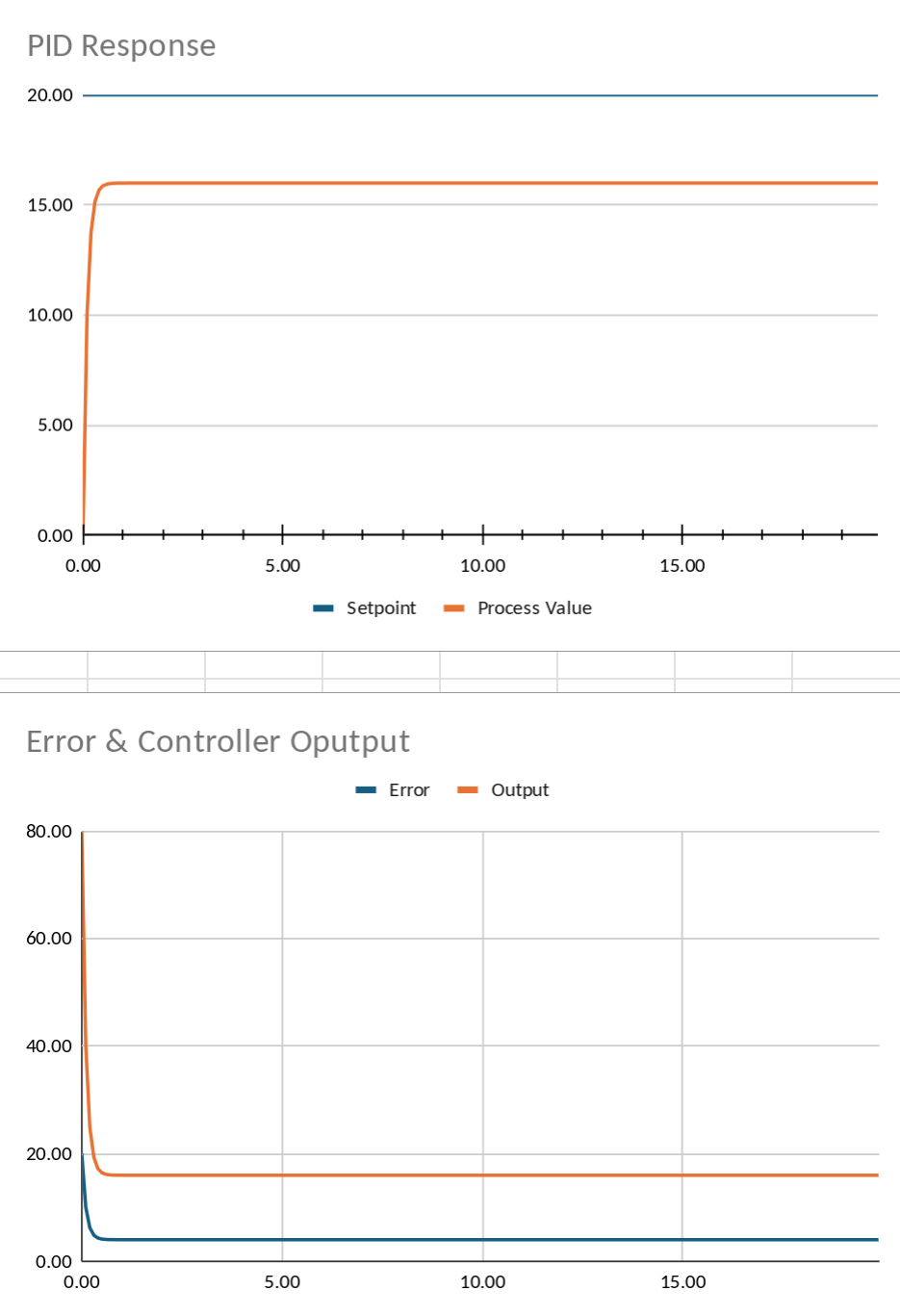
Watch where it eventually settles. With the suggested values, the process value winds up around 16 even though our setpoint is 20. Why? At a process value of 20, the error would be zero. A proportional controller presented with zero error produces zero output. But this particular process needs an output of 20 to remain at 20. Therefore, it can’t ever quite get there.
This is the classic steady-state error of proportional-only control. We could crank Kp upward. Try Kp=8. The process gets much closer to the setpoint. But continually increasing proportional gain isn’t a universal solution. Eventually real systems start overshooting, oscillating, amplifying noise, or otherwise expressing their displeasure. We need another term.
Remember the Error
Set Kp back to 4 and try:
Ki = 0.5
The integral term looks at not just the error right now, but the error accumulated over time. In the spreadsheet there’s an Integral State column. Each row does approximately this:
integral = previous_integral + error × dt
and the I contribution becomes:
I = Ki × integral
Now consider our P controller sitting stubbornly below the desired value. As long as some positive error remains, the integral keeps growing.
That gradually increases the controller output until the remaining error disappears. Instead of settling around 16, the process now creeps all the way toward 20. This demonstrates one of the major reasons integral control exists: it eliminates persistent offset. It also gives us a good excuse to disturb the system.
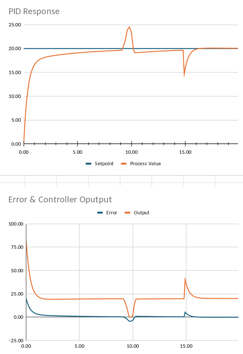
Select the user process model and set User Model # to 1. This will let you disturb the process value by entering numbers into the User1 column. Leave the first bit of the User1 column at 0. But somewhere farther down the simulation, put a disturbance into that column — perhaps -5. If you are feeling especially salty, try a sequence like: 0.5, 0.75, 1, 1.5, 2, 1.5, 0.75, 0.5, -1, -1, -0.5. That sequence should already be in the template’s User1 column.
You can imagine that as opening a refrigerator door, suddenly putting a mechanical load on a motor, or connecting another load to a regulated power supply.
A proportional-only controller reacts immediately, but once things settle, it again tolerates a permanent error.
The integral controller doesn’t. If the process remains below the setpoint, integral action continues increasing until the disturbance has been compensated. That’s a powerful trick. Unfortunately, integral control has tricks of its own.
Too Much of a Good Thing
Integral action remembers errors, but memories aren’t always helpful. The derivative term responds to how rapidly the error is changing:
D = Kd × (error - previous_error) / dt
If proportional control asks, “How far away are we?”, derivative control asks, “How fast are we approaching?” Or, more precisely in this case, “How fast is the error changing?”
Make the simulated process faster by changing its time constant from 2 to about 0.8 seconds. Then try something deliberately more aggressive:
Kp = 8
Ki = 1
Kd = 0
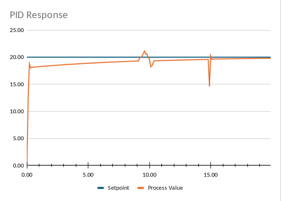
The response now gets to the setpoint quickly, but it overshoots it. The problem is easy to see in the spreadsheet. While the process is racing upward, it remains below the setpoint, so the integral continues accumulating positive error. By the time we arrive at the destination, the integral term is still pushing. Depending on the process and gains, the result may be a little overshoot, a lot of overshoot, or sustained oscillation.
Since the default plant is only first-order, derivative action doesn’t have much to work with. User Model 2 adds another lag, using the USER2 column as an intermediate process state. That produces more phase lag and makes aggressive PI tuning more prone to overshoot.
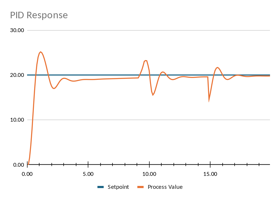
Switch to User Model 2 and start with Kd=0. Then note the peak process value. Then try Kd=0.2, 0.5, and perhaps 1.0. Try some negative values. You will find that there is a range where the peak overshoot is reduced slightly, but keep going and the response starts to ring. Push Kd far enough, and the derivative term becomes part of the problem rather than part of the cure. The graphs autoscale, so sometimes what looks like a peak the same size (or even bigger) is really smaller than the previous result. Be sure to read the numbers.
That’s the basic PID balancing act. P reacts to the error that exists now. I reacts to error that has existed for a while. D reacts to where the error appears to be heading. Put all three together, and you have a controller that may respond strongly, eliminate steady-state error, and anticipate rapid changes. However, sometimes you are better off with, for example, just PI or even just pure proportional control. Having the algorithm in a spreadsheet form is a nice way to experiment, especially if you can model the system’s behavior.
It’s Only a Spreadsheet
You can add your own models by modifying USR_PROCESS to call your function or just modify one of the existing ones. DEF_PROCESS is just a simple lag model. USR_PROCESS0 has some random noise, while USR_PROCESS1 lets you inject a disturbance in the USER1 column. USR_PROCESS2 is like USR_PROCESS1 but has a second-order process in the USER2 column as well. Of course, real control systems are messier than these nice models.
The output may have hard limits. In fact, the spreadsheet includes minimum and maximum output clamps. This exposes another classic PID problem: integral windup. If the controller desperately requests an output of 150 but the actuator can only deliver 100, the integral can continue accumulating error even though the actuator cannot respond. When the error finally reverses, all of that stored integral has to unwind. Practical controllers frequently include anti-windup schemes to deal with this. In practical terms, imagine a thermistor gets unplugged, and the system suddenly thinks there is a giant temperature error. It will try to correct it, but it can’t. Then someone plugs the sensor back in. All the accumulated error in the integral term now has to be backed off.
Derivative action causes its own problems. The spreadsheet calculates derivative from the error, which means suddenly changing the setpoint produces a large derivative pulse — the notorious derivative kick. Real controllers often calculate derivative from the process value instead.
Of course, real measurements also contain noise. Differentiation is very good at making high-frequency noise more prominent, so the D term is commonly filtered. We aren’t doing any of those sophisticated things here, and that’s intentional. The point of the sheet is that every number is visible and to make it easy to experiment.
Change a setpoint in the middle of the Setpoint column, and you’ve generated a step input. Change one of the User columns, and you can inject a disturbance. Adjust Kp, Ki, or Kd, and you can immediately see which portions of the controller output changed and why.
To add your own models, modify USR_PROCESS and add a custom function to the SWITCH statement. Then create your custom function. If you need to grab data from the spreadsheet, you’ll see examples of using ROW() and INDIRECT() to get the right numbers. It is fairly straightforward to add motors, thermal systems, second-order plants, dead time, nonlinearities, or whatever other pathological system you’d like to inflict on your controller.
The most important lesson about PID control? There isn’t a magic set of Kp, Ki, and Kd values. A set of gains that works beautifully on one plant may be terrible on another. Change the mass, thermal capacity, load, delay, sample rate, actuator limits, or sensor characteristics and the optimum controller changes with it. Not every control job needs all three terms.
The equations fit comfortably into a few spreadsheet cells. The interesting part is figuring out what numbers to put in them.
Most of our spreadsheet hijinks center around DSP. Except for the ones that simulate computers.









PID is primitive caveman compared to something like LQR, but to understand it you need university education. YouTube video won’t do it.
Yes, definitely need a “university education” to understand such things. YouTube videos are only intended for the lower class, unclean, peasants & serfs. They can’t be expected to grasp “university” level subjects like our superior social class.
Pardon me, do you have some Grey Poupon ?
I’ve always preferred English Mustard myself.
I know, how boring mundane of me. Sadly this is the result of attending an English Public School and not an ‘up market’ U.S. college :)
what kind of bad/simple schools/universities do you have if LQR is universisty level?
PID is a good choice for a temperature sensor or a servo. PID is not a good choice for the multi-axis controls of a CNC (especially when you have to mix linear XYZ movement with some rotational movements). I would argue that LQR is of a moderate university level, but only entry-level if your university coursework is for robotics.
what about ADRC? I want to experiment with it soon
Of interest
https://techxplore.com/news/2026-07-ai-framework-rooted-cognitive-science.html
Works well in excel too.
If you need help in PID tuning get a step response and enter it in https://pidtuner.github.io
Let’s say I’m trying to control a process that frequently changes things like load, delay and thermal capacity and don’t want to mess with the pid every time. Is there a better method?
I’ve modified my older catalytic wood burning stove to be controlled by an esp32 and thermocouples measuring the catalytic temp, stove top and flue. There are numerous safety features and redundancies, of course. All tested in a controlled enviroment because I like having a house. The process is controlled by restricting airflow with a servo moving a butterfly valve with seals.
My issue is that it has proven impossible to tune out oscillating over and undershooting the target. Things like ambient temperature, wood moisture levels, wood species/size/quantity/the way it is stacked in the stove, ash levels in the stove, wind all seem to change the ideal pid settings.
While it works wonderfully as it is currently I always wonder if it could work even better. I’ve got it down to oscillations of, typically, +/- 20 degrees, sometimes as bad as +/- 100 degrees. Normal operating temp is 1000 to 1600 degrees.
Is there a control scheme that is more fitting for this use?
I’m definitely no expert, but I’d guess you’d be best served by adding an oxygen sensor in the flue, like you’d find in a car’s exhaust. Possibly followed by a pair of hygrometers on the intake and the flue. So your system could have more direct awareness of the state of the fire.
I’ve pondered this a bit. I have set up a similar system with my wood stove (although probably not as thorough as yours) and have experienced a similar issue. My best guess is something like model predictive control. At least on my stove, there is a good 1-2 minutes between any adjustment to the air control and resulting behavior, which is really hard for PID to deal with. If the controller had a model of the system it could predict how the current adjustment would affect the trajectory, and not just respond to the past.
I’d love to see more of your setup! Have you written any of it up?
Have you tried something like a Kalman filter? Maybe it simply loses accuracy due to noise in the system. I often used it in micro mouse competitions.
MORE PID
Spreadsheets are underused in electronics.
I’ve been modeling pid’s, circuits (especially non-linear ones) and a host of other things for 30 years now in spreadsheets. Set dT smaller until things don’t change.
Great fun, and a useful tool.
Its true. I’ve been in the spreadsheet camp firmly for as long as I can remember although I was enchanted by the python (numpy+pandas+matplotlib+pywidgets) camp for a while. The ease of use of spreadsheets is its biggest strength.
Python can be immensely useful though if you want to build a model or do stuff with any kind of numeric data that is stored in a file, and can be swapped out. Also array operations. Python is good at that
Apparently not mentioned here but VERY important… what happens when you have an integrative process, something like DC motor position where what you have control of (torque at a given moment) gets integrated over time (in some systems integrated multiple times torque–>speed–>position) to give the value you’re actually trying to control. That’s what I’d like to hear more about.
Niche fields of study are finding greater use:
https://techxplore.com/news/2026-08-negative-imaginary-theory-math-niche.html
NI will help reduce vibration issues, one hopes.
Doing PID with a 555 timer is more interesting and a lot more practical for projects.
Could you please elaborate or provide an example? I’m intrigued.
Error → Split → [P path → 555] → \
→ [I path → RC → 555] → >— Summing → MOSFET → Load
→ [D path → RC → 555] → /
Course my ASCII art always sucks.
interesting sheet, is there any way to download a copy?
Setting up a sin wave input will give more insight into a control process.
also there are two forms of the differential term. using error slope gives a reactive response while using command slope gives a predictive response.
You should be able to load it then “Save As” into your account.
No Save As option under File menu