$Two very similar diffraction patterns are shown, in patterns of green dots against a blue background. The left image is labelled "Kompressions-algorithmus", and the one on the right is labelled "Licht & Zweibelzellen".$

Why Diffraction Gratings Create Fourier Transforms

January 27, 2026 by Aaron Beckendorf 9 Comments

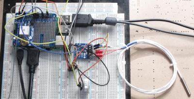
When last we saw [xoreaxeax], he had built a lens-less optical microscope that deduced the structure of a sample by recording the diffraction patterns formed by shining a laser beam through it. At the time, he noted that the diffraction pattern was a frequency decomposition of the specimen’s features – in other terms, a Fourier transform. Now, he’s back with an explanation of why this is, deriving equations for the Fourier transform from the first principles of diffraction (German video, but with auto-translated English subtitles. Beware: what should be “Huygens principle” is variously translated as “squirrel principle,” “principle of hearing,” and “principle of the horn”).

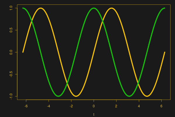
The first assumption was that light is a wave that can be adequately represented by a sinusoidal function. For the sake of simplicity (you’ll have to take our word for this), the formula for a sine wave was converted to a complex number in exponential form. According to the Huygens principle, when light emerges from a point in the sample, it spreads out in spherical waves, and the wave at a given point can therefore be calculated simply as a function of distance. The principle of superposition means that whenever two waves pass through the same point, the amplitude at that point is the sum of the two. Extending this summation to all the various light sources emerging from the sample resulted in an infinite integral, which simplified to a particular form of the Fourier transform.

One surprising consequence of the relation is the JPEG representation of a micrograph of some onion cells. JPEG compression calculates the Fourier transform of an image and stores it as a series of sine-wave striped patterns. If one arranges tiles of these striped patterns according to stripe frequency and orientation, then shades each tile according to that pattern’s contribution to the final image, one gets a speckle pattern with a bright point in the center. This closely resembles the diffraction pattern created by shining a laser through those onion cells.

For the original experiment that generated these patterns, check out [xoreaxeax]’s original ptychographical microscope. Going in the opposite direction, researchers have also used physical structures to calculate Fourier transforms.

Continue reading “Why Diffraction Gratings Create Fourier Transforms” →

Sensor Filters For Coders

September 6, 2019 by Pat Whetman 35 Comments

Anybody interested in building their own robot, sending spacecraft to the moon, or launching inter-continental ballistic missiles should have at least some basic filter options in their toolkit, otherwise the robot will likely wobble about erratically and the missile will miss it’s target.

What is a filter anyway? In practical terms, the filter should smooth out erratic sensor data with as little time lag, or ‘error lag’ as possible. In the case of the missile, it could travel nice and smoothly through the air, but miss it’s target because the positional data is getting processed ‘too late’. The simplest filter, that many of us will have already used, is to pause our code, take about 10 quick readings from our sensor and then calculate the mean by dividing by 10. Incredibly simple and effective as long as our machine or process is not time sensitive – perfect for a weather station temperature sensor, although wind direction is slightly more complicated. A wind vane is actually an example of a good sensor giving ‘noisy’ readings: not that the sensor itself is noisy, but that wind is inherently gusty and is constantly changing direction.

It’s a really good idea to try and model our data on some kind of computer running software that will print out graphs – I chose the Raspberry Pi and installed Jupyter Notebook running Python 3.

The photo on the left shows my test rig. There’s a PT100 probe with it’s MAX31865 break-out board, a Dallas DS18B20 and a DHT22. The shield on the Pi is a GPS shield which is currently not used. If you don’t want the hassle of setting up these probes there’s a Jupyter Notebook file that can also use the internal temp sensor in the Raspberry Pi. It’s incredibly quick and easy to get up and running.

It’s quite interesting to see the performance of the different sensors, but I quickly ended up completely mangling the data from the DS18B20 by artificially adding randomly generated noise and some very nasty data spikes to really punish the filters as much as possible. Getting the temperature data to change rapidly was effected by putting a small piece of frozen Bockwurst on top of the DS18B20 and then removing it again.

Continue reading “Sensor Filters For Coders” →

Imaginary AC Circuits Aren’t Really Complex

June 15, 2017 by Al Williams 32 Comments

If you have ever read advanced textbooks or papers about electronics, you may have been surprised to see the use of complex numbers used in the analysis of AC circuits. A complex number has two parts: a real part and an imaginary part. I’ve often thought that a lot of books and classes just kind of gloss over what this really means. What part of electricity is imaginary? Why do we do this?

The short answer is phase angle: the time delay between a voltage and a current in a circuit. How can an angle be a time? That’s part of what I’ll need to explain.

First, consider a resistor. If you apply a voltage to it, a certain current will flow that you can determine by Ohm’s law. If you know the instantaneous voltage across the resistor, you can derive the current and you can find the power–how much work that electricity will do. That’s fine for DC current through resistors. But components like capacitors and inductors with an AC current don’t obey Ohm’s law. Take a capacitor. Current only flows when the capacitor is charging or discharging, so the current through it relates to the rate of change of the voltage, not the instantaneous voltage level.

That means that if you plot the sine wave voltage against the current, the peak of the voltage will be where the current is minimal, and the peak current will be where the voltage is at zero. You can see that in this image, where the yellow wave is voltage (V) and the green wave is current (I). See how the green peak is where the yellow curve crosses zero? And the yellow peak is where the green curve crosses zero?

These linked sine and cosine waves might remind you of something — the X and Y coordinates of a point being swept around a circle at a constant rate, and that’s our connection to complex numbers. By the end of the post, you’ll see it isn’t all that complicated and the “imaginary” quantity isn’t imaginary at all.

Continue reading “Imaginary AC Circuits Aren’t Really Complex” →