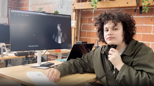
Speak Silently With An Ultrasound Probe

July 12, 2026 by Donald Papp 14 Comments

Speaking is much faster than typing, and while it’s an increasingly convenient way to interact with computers, it’s hardly private. Providing speech privacy in a way we haven’t seen before is this prototype tongue-reading system that uses machine learning and ultrasound to read tongue movements and turn them into decoded speech. Not only can a user speak without emitting a sound, since it doesn’t read sound waves it’s completely immune to noisy environments.

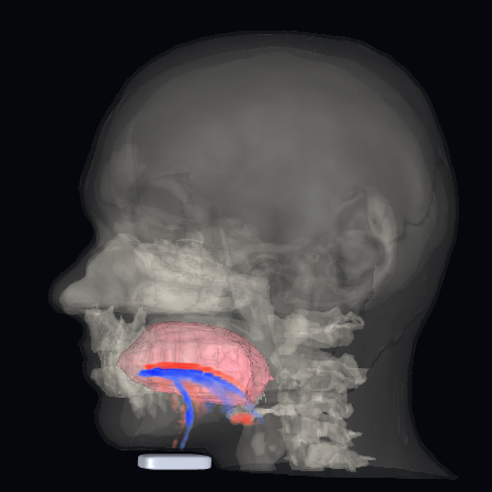
Tongues are a far richer source of speech data than reading lip and mouth movements.

It turns out that tongue movements are a very rich source of information about speech, and an ultrasound probe under the chin takes very clear video of a tongue. With a dataset consisting of only around 50 hours of training data, the system has a 15.6% error rate and generalizes across different speakers (as long as they speak with similar accents).

That error rate may seem high at first glance, but keep in mind this is for a prototype system built in a month around a relatively small training dataset. All indications are that better results are just a matter of better training.

Probably the biggest drawback at the moment is the size of the ultrasound probe and the way it must be held under one’s chin like a contact microphone, but at the moment the probe is an off-the-shelf model that is hardly optimized for either size, weight, or wearability. If the system seems promising enough, a probe resembling an adhesive patch might even be possible.

It’s certainly a different approach from others we’ve seen in the past, including whispering while inhaling and reading lip and mouth movements.

Teaching An AI To Play A Racing Game Via Screen Input

June 28, 2026 by Zoe Skyforest 2 Comments

If you’re a fleshy human, you probably learn to play video games by looking at the screen and pressing the buttons, and maybe copying the way you’ve seen others play the game before. [tryfonaskam] has recently been trying to teach an AI to play games in much the same way.

[tryfonaskam] built PILA—short for Polytrack Imitation Learning Agent. As you might have guest from the name, it’s an AI agent designed to play a simple racing game called PolyTrack. Rather than manually programming the agent’s behavior, PILA instead trains itself through supervised learning, where it observes the gameplay state via screen capture and monitoring the keyboard inputs made by human players as they drive the tracks. It then uses this to guide its own behavior, and learns to play the game by itself. The model receives live frames from the graphics engine while playing, and then predicts the appropriate actions and makes the right keyboard inputs in turn to steer the car through the track.

This project reminds us of similar efforts to teach a raw AI how to play Trackmania, or the Drivatar technology in the Forza series of racing games.

Training A Transformer With 1970s-era Technology

March 29, 2026 by Bryan Cockfield 15 Comments

Although generative language models have found little widespread, profitable adoption outside of putting artists out of work and giving tech companies an easy scapegoat for cutting staff, their their underlying technology remains a fascinating area of study. Stepping back to the more innocent time of the late 2010s, before the cultural backlash, we could examine these models in their early stages. Or, we could see how even older technology processes these types of machine learning algorithms in order to understand more about their fundamentals. [Damien Boureille] has put a 60s-era IBM as well as a PDP-11 to work training a transformer algorithm in order to take a closer look at it.

For such old hardware, the task [Damien Boureille] is training his transformer to do is to reverse a list of digits. This is a trivial problem for something like a Python program but much more difficult for a transformer. The model relies solely on self-attention and a residual connection. To fit within the 32KB memory limit of the PDP-11, it employs fixed-point arithmetic and lookup tables to replace computationally expensive functions. Training is optimized with hand-tuned learning rates and stochastic gradient descent, achieving 100% accuracy in 350 steps. In the real world, this means that he was able to get the training time down from hours or days to around five minutes.

Not only does a project like this help understand these tools, but it also goes a long way towards demonstrating that not every task needs a gigawatt datacenter to be useful. In fact, we’ve seen plenty of large language models and other generative AI running on computers no more powerful than an ESP32 or, if you need slightly more computing power, on consumer-grade PCs with or without GPUs.

Repurposing Old AMD APUs For AI Work

March 18, 2026 by Zoe Skyforest 22 Comments

The BC250 is what AMD calls an APU, or Accelerated Processing Unit. It combines a GPU and CPU into a single unit, and was originally built to serve as the heart of certain Samsung rack mount servers. If you know where to find cheap surplus units of the BC250, you can put them to good use for AI work, as [akandr] demonstrates.

The first thing you’ll have to figure out is how to take an individual BC250 APU and get it up and running. It’s effectively a full system-on-chip, combining a Zen 2 CPU with a Cyan Skillfish RDNA 1.5 GPU. However, it was originally intended to run inside a rackmount server unit rather than a standalone machine. To get it going, you’ll need to hook it up with power and some kind of cooling solution.

From there, it’s a matter of software. [akandr] explains how to get AI workflows running on the BC250 using Ollama and Vulkan, while noting useful hacks to improve performance like disabling the GUI and tweaking the CPU governor. The hardware can be used with a wide range of different models depending on what you’re trying to achieve, it just takes some careful management of the APU’s resources to get the most out of it. Thankfully, that’s all in the guide on GitHub.

We’ve already seen these AMD APUs repurposed before for gaming use. Unfortunately the word is out already about their capabilities, so prices have risen significantly in response to demand. Still, if you manage to score a BC250 and do something cool with it yourself, be sure to let us know on the tipsline!

DIY Wall-Plotter Does Generative Art, But Not As We Know It

February 11, 2026 by Donald Papp No comments

[Teddy Warner]’s GPenT (Generative Pen-trained Transformer) project is a wall-mounted polargraph that makes plotter art, but there’s a whole lot more going on than one might think. This project was partly born from [Teddy]’s ideas about how to use aspects of machine learning in ways that were really never intended. What resulted is a wall-mounted pen plotter that offers a load of different ‘generators’ — ways to create line art — that range from procedural patterns, to image uploads, to the titular machine learning shenanigans.

There are loads of different ways to represent images with lines, and this project helps explore them.

Want to see the capabilities for yourself? There’s a publicly accessible version of the plotter interface that lets one play with the different generators. The public instance is not connected to a physical plotter, but one can still generate and preview plots, and download the resulting SVG file or G-code.

Most of the generators do not involve machine learning, but the unusual generative angle is well-represented by two of them: dcode and GPenT.

dcode is a diffusion model that, instead of converting a text prompt into an image, has been trained to convert text directly into G-code. It’s very much a square peg in a round hole. Visually it’s perhaps not the most exciting, but as a concept it’s fascinating.

The titular GPenT works like this: give it a scrap of text inspiration (a seed, if you will), and that becomes a combination of other generators and parameters, machine-selected and stacked with one another to produce a final composition. The results are unique, to say the least.

Once the generators make something, the framed and wall-mounted plotter turns it into physical lines on paper. Watch the system’s first plot happen in the video, embedded below under the page break.

This is a monster of a project representing a custom CNC pen plotter, a frame to hold it, and the whole software pipeline both for the CNC machine as well as generating what it plots. Of course, the journey involved a few false starts and dead ends, but they’re all pretty interesting. The plotter’s GitHub repository combined with [Teddy]’s write up has all the details one may need.

It’s also one of those years-in-the-making projects that ultimately got finished and, we think, doing so led to a bit of a sigh of relief on [Teddy]’s part. Most of us have unfinished projects, and if you have one that’s being a bit of a drag, we’d like to remind you that you don’t necessarily have to finish-finish a project to get it off your plate. We have some solid advice on how to (productively) let go.

Continue reading “DIY Wall-Plotter Does Generative Art, But Not As We Know It” →

AI Picks Outfits With Abandon

December 17, 2025 by Zoe Skyforest 4 Comments

Most of us choose our own outfits on a daily basis. [NeuroForge] decided that he’d instead offload this duty to artificial intelligence — perhaps more for the sake of a class project than outright fashion.

The concept involved first using an AI model to predict the weather. Those predictions would then be fed to a large language model (LLM), which would recommend an appropriate outfit for the conditions. The output from the LLM would be passed to a simple alarm clock which would wake [NeuroForge] and indicate what he should wear for the day. Amazon’s Chronos forecasting model was used for weather prediction based on past weather data, while Meta’s Llama3.1 LLM was used to make the clothing recommendations. [NeuroForge] notes that it was possible to set all this up to work without having to query external services once the historical weather data had been sourced.

While the AI choices often involved strange clashes and were not weather appropriate, [NeuroForge] nonetheless followed through and wore what he was told. This got tough when the outfit on a particularly cold day was a T-shirt and shorts, though the LLM did at least suggest a winter hat and gloves be part of the ensemble. Small wins, right?

We’ve seen machine learning systems applied to wardrobe-related tasks before. One wonders if a more advanced model could be trained to pick not just seasonally-appropriate clothes, but to also assemble actually fashionable outfits to boot. If you manage to whip that up, let us know on the tipsline. Bonus points if your ML system gets a gig on the reboot of America’s Next Top Model.

Continue reading “AI Picks Outfits With Abandon” →

Why LLMs Are Less Intelligent Than Crows

December 10, 2025 by Maya Posch 61 Comments

The basic concept of human intelligence entails self-awareness alongside the ability to reason and apply logic to one’s actions and daily life. Despite the very fuzzy definition of ‘human intelligence‘, and despite many aspects of said human intelligence (HI) also being observed among other animals, like crows and orcas, humans over the ages have always known that their brains are more special than those of other animals.

Currently the Cattell-Horn-Carroll (CHC) theory of intelligence is the most widely accepted model, defining distinct types of abilities that range from memory and processing speed to reasoning ability. While admittedly not perfect, it gives us a baseline to work with when we think of the term ‘intelligence’, whether biological or artificial.

This raises the question of how in the context of artificial intelligence (AI) the CHC model translate to the technologies which we see in use today. When can we expect to subject an artificial intelligence entity to an IQ test and have it handily outperform a human on all metrics?

Continue reading “Why LLMs Are Less Intelligent Than Crows” →