This week on the Podcast, we have something a little different for you. Elliot is on vacation, so Tom was in charge of running the show and he had Kristina in the hot seat.
 First up in the news: the 2024 Tiny Games Challenge is still underway and has drawn an impressive 44 entries as of this writing. You have until 9AM PDT on September 10th to show us your best tiny game, whether that means tiny hardware, tiny code, or a tiny BOM.
Then it’s on to What’s That Sound, which Tom and Kristina came up with together, so there will be no pageantry about guessing. But can you get it? Can you figure it out? Can you guess what’s making that sound? If you can, and your number comes up, you get a special Hackaday Podcast t-shirt.
Now it’s on to the hacks, beginning with an open-source liquid-fueled rocket and a really cool retro trackball laptop. Then we’ll discuss screwdriver mange, the Wow! signal, and whether you’re using you’re calipers incorrectly. Finally, we look at a laptop that that isn’t really a laptop, and one simple trick to keep things aligned on your laser engraver.
Check out the links below if you want to follow along, and as always, tell us what you think about this episode in the comments!
Download in DRM-free MP3 and savor at your leisure.