Just a few weeks before Atlantis embarked on the final flight of the Space Shuttle program in 2011, a small Mexican company by the name of Squad quietly released Kerbal Space Program (KSP) onto an unsuspecting world. Until that point the company had only developed websites and multi-media installations. Kerbal wasn’t even an official company initiative, it started as a side project by one of their employees, Felipe Falanghe. The sandbox game allowed players to cobble together rockets from an inventory of modular components and attempt to put them into orbit around the planet Kerbin. It was immediately addictive.
There was no story to follow, or enemies to battle. The closest thing to a score counter was the altimeter that showed how far your craft was above the planet’s surface, and the only way to “win” was to put its little green occupant, the titular Kerbal, back on the ground in one piece. The game’s challenge came not from puzzles or scripted events, but from the game’s accurate (if slightly simplified) application of orbital mechanics and Newtonian dynamics. Building a rocket and getting it into orbit in KSP isn’t difficult because the developers baked some arbitrary limitations into their virtual world; the game is hard for the same reasons putting a rocket into orbit around the Earth is hard.
One of my early rockets, circa 2013.
Over the years official updates added new components for players to build with and planets to explore, and an incredible array of community developed add-ons and modifications expanded the scope of the game even further. KSP would go on to be played by millions, and seeing a valuable opportunity to connect with future engineers, both NASA and the ESA helped develop expansions for the game that allowed players to recreate their real-world vehicles and missions.
But now after a decade of continuous development, with ports to multiple operating systems and game consoles, Squad is bringing this chapter of the KSP adventure to a close. To celebrate the game’s 10th anniversary on June 24th, they released “On Final Approach”, the game’s last official update. Attention will now be focused on the game’s ambitious sequel, which will expand the basic formula with the addition of interstellar travel and planetary colonies, currently slated for release in 2022.
Of course, this isn’t the end. Millions of “classic” KSP players will still be slinging their Kerbals into Hohmann transfer orbits for years to come, and the talented community of mod developers will undoubtedly help keep the game fresh with unofficial updates. But the end of official support is a major turning point, and it seems a perfect time to reminisce on the impact this revolutionary game has had on the engineering and space communities.
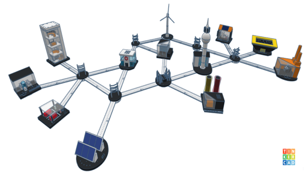
The electric power grid, as it exists today, was designed about a century ago to accommodate large, dispersed power plants owned and controlled by the utilities themselves. At the time this seemed like a great idea, but as technology and society have progressed the power grid remains stubbornly rooted in this past. Efforts to modify it to accommodate solar and wind farms, electric cars, and other modern technology need to take great effort to work with the ancient grid setup, often requiring intricate modeling like this visual power grid emulator.
The model is known as LEGOS, the Lite Emulator of Grid Operations, and comes from researchers at RWTH Aachen University. Its goal is to simulate a modern power grid with various generation sources and loads such as homes, offices, or hospitals. It uses a DC circuit to simulate power flow, which is visualized with LEDs. The entire model is modular, so components can be added or subtracted easily to quickly show how the power flow changes as a result of modifications to the grid. There is also a robust automation layer to the entire project, allowing real-time data acquisition of the model to be gathered and analyzed using an open source cloud service called FIWARE.
In order to modernize the grid, simulations like these are needed to make sure there are no knock-on effects of adding or changing such a complex system in ways it was never intended to be changed. Researchers in Europe like the ones developing LEGOS are ahead of the curve, as smart grid technology continues to filter in to all areas of the modern electrical infrastructure. It could also find uses for modeling power grids in areas where changes to the grid can happen rapidly as a result of natural disasters.
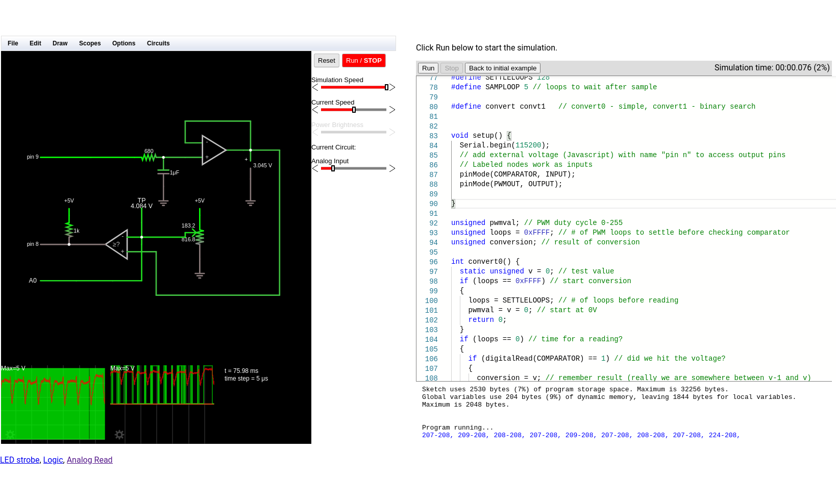
There was a time when building electronics and building software were two distinct activities. These days, almost any significant electronic project will use a CPU somewhere, or — at least — could. Using a circuit simulator can get you part of the way and software simulators abound. But cosimulation — simulating both analog circuits and a running processor — is often only found in high-end simulation products. But I noticed the other day the feature quietly snuck into our favorite Web-based simulator, Falstad.
The classic simulator is on the left and the virtual Arduino is on the right.
Back in March, the main project added work from [Mark McGarry] to support AVR8js written by [Uri Shaked]. The end result is you can have the circuit simulator on the left of the screen and a Web-based Arduino IDE on the right side. But how does it work beyond the simple demo? We wanted to find out.
The screen looks promising. The familiar simulator is to the left and the Arduino IDE — sort of — is to the right. There’s serial output under the source code, but it doesn’t scroll very well, so if you output a lot of serial data, it is hard to read.
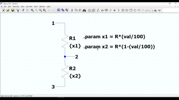
If you enjoy simulating circuits, you’ve probably used LTSpice. The program has a lot of powerful features we tend to not use, including the ability to make custom components that are quite complex. To illustrate how it works, [asa pro] builds a potentiometer component that is not only a good illustration but also a useful component.
The component is, of course, just two resistors. However, using parameters, the component gets two values, a total resistance and a percentage. Then the actual resistance values adjust themselves.
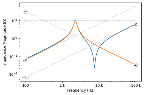
Using circuit simulating software like SPICE can be a powerful tool for modeling the behavior of a circuit in the real world. On the other hand, it’s not always necessary to have all of the features of SPICE available all the time, and these programs tend to be quite expensive as well. To that end, [Wes Hileman] noticed an opportunity for a specific, quick method for performing impedance calculations using python without bulky, expensive software and came up with a program which he calls fastZ.
The software works on any network of passive components (resistors, capacitors, and inductors) and the user can specify parallel and series connections using special operators. Not only can the program calculate the combined impedance but it can perform frequency analysis at a specified frequency or graph the frequency response over a wide range of frequencies. It’s also running in python which makes it as simple as importing any other python package, and is also easy to implement in any other python program compared to building a simulation and hoping for the best.
If you find yourself regularly drawing Bode plots or trying to cobble together a circuit simulation to work with your python code, this sort of solution is a great way to save a lot of headache. It is possible to get the a piece of software like SPICE to to work together with other python programs though, often with some pretty interesting results.
[Everett]’s 5-year-old loves a simple game called Hoot Owl Hoot! in which players cooperatively work to move owls along a track to the safety of a nest. Player pieces move on spaces according to the matching colors drawn from a deck of cards. If a space is already occupied, a piece may jump ahead to the next available spot. The game has a bit more to it than that, but those are the important parts. After a few games, the adults in the room found themselves disagreeing about which strategy was optimal in this simple game.
It seemed to [Everett] that it was best to move pieces in the rear, keeping player pieces grouped together and maximizing the chance of free moves gained by jumping over occupied spaces. [Everett]’s wife countered that a “longest move” strategy was best, and one should always select whichever piece would benefit the most (i.e. move the furthest distance) from any given move. Which approach wins games in the fewest moves? This small Python script simulates the game enough to iteratively determine that the two strategies are quite close in results, but the “longest move” strategy does ultimately come out on top.
As far as simulations go, it’s no Tamagotchi Singularity and [Everett] admits that the simulation isn’t a completely accurate one. But since its only purpose is to compare whether “no stragglers” or “longest move” wins in fewer moves, shortcuts like using random color generation in place of drawing the colors from a deck shouldn’t make a big difference. Or would it? Regardless, we can agree that board games can be fitting metaphors for the human condition.
Circuit simulations are great because you can experiment with circuits and make changes with almost no effort. In Circuit VR, we look at circuits using a simulator to do experiments without having to heat up a soldering iron or turn on a bench supply. This time, we are going to take a bite of a big topic: op amps.
The op amp — short for operational amplifier — is a packaged differential amplifier. The ideal op amp — which we can’t get — has infinite gain and infinite input impedance. While we can’t get that in real life, modern devices are good enough that we can pretend like it is true most of the time.
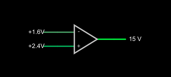
a very simple op amp circuit with some detail omitted
If you open this circuit in the Falstad simulator, you’ll see two sliders to the right where you can tweak the input voltage. If you make the voltages the same, the output will be zero volts. You might think that a difference amplifier would take inputs of 1.6V and 2.4V and either produce 0.8V or -0.8V, but that’s not true. Try it. Depending on which input you set to 2.4V, you’ll get either 15V or -15V on the output. That’s the infinite gain. Any positive or negative output voltage will quickly “hit the rail” or the supply voltage which, in this case, is +/-15V.
Practical Concerns
The biggest omitted detail in the schematic symbol above is that there’s no power supply here, but you can guess that it is +/- 15V. Op amps usually have two supplies, a positive and a negative and while they don’t have to be the same magnitude, they often are. Some op amps are specifically made to work with a single-ended supply so their negative supply can connect to ground. Of course, that presupposes that you don’t need a negative voltage output.
The amount of time it takes the output to switch is the slew rate and you’ll usually find this number on the device datasheet. Obviously, for high-speed applications, a fast slew rate is important, particularly if you want to use the circuit as a comparator as we are here.
Other practical problems arise because the op amp isn’t really perfect. A real op amp would not hit the 15V rail exactly. It will get close depending on how much current you draw from the output. The higher the current, the further away from the rails you get. Op amps will also have some offset that will prevent it from hitting zero when the inputs are equal, although on modern devices that can be very low. Some older devices or those used in high-precision designs will have a terminal to allow you to trim the zero point exactly using an external resistor.
Op Amps Can Provide Steady Voltage Under Variable Load
Rather than dig through a lot of math, you can deal with nearly all op amp circuits if you remember two simple rules:
The inputs of the op amp don’t connect to anything internally.
The output mysteriously will do what it can to make the inputs equal, as far as it is physically possible.
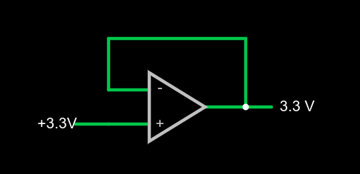
1x amplifier
That second rule will make more sense in a minute, but we already see it in action. Set the simulator so the – input (the inverting input) is at 0V and the noninverting input (+) is at 4V. The output should be 15V. The output is trying to make the inverting input match the noninverting one, but it can’t because there is no connection. The output would like to provide an infinite amount of voltage, but it can only go up to the rail which is 15V.
We can exploit this to make a pretty good x1 amplifier by simply shorting the output to the – terminal. Remember, our rules say the input terminals appear to not connect to anything, so it can’t hurt. Now the amplifier will output whatever voltage we put into it:
You might wonder why this would be interesting. Well, we will learn how to increase the gain, but you actually see this circuit often enough because the input impedance is very high (infinite in theory, but not practice). And the output impedance is very low which means you can draw more current without disturbing the output voltage much.
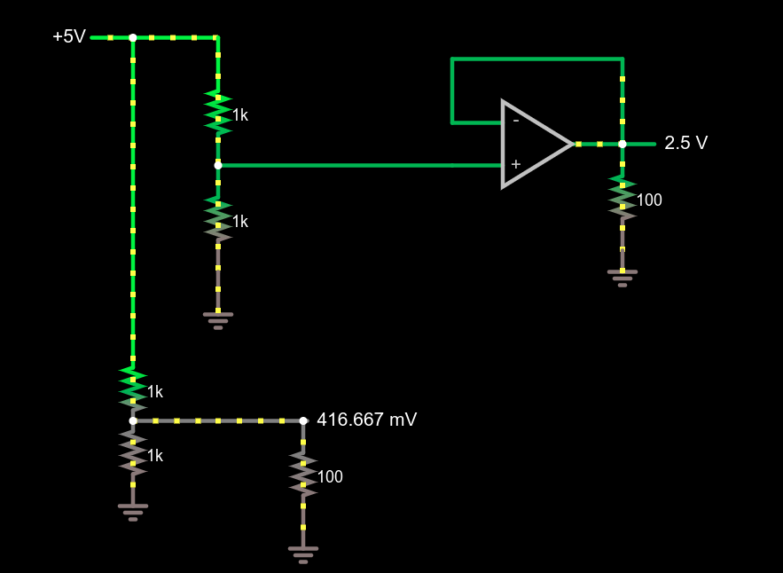
Comparing voltage divider performance with and without a 1x amplifier
This circuit demonstrates the power of a 1x amplifier. Both voltage dividers produce 2.5V with no load. However, with a 100 ohm load at the output, the voltage divider can only provide around 400mV. You’d have to account for the loading in the voltage divider design and if the load was variable, it wouldn’t be possible to pick a single resistor that worked in all cases. However, the top divider feeds the high impedance input of the op amp which then provides a “stiff” 2.5V to whatever load you provide. As an example, try changing the load resistors from 100 ohms to different values. The bottom load voltage will swing wildly, but the top one will stay at 2.5V.
Don’t forget there are practical limits that won’t hold up in real life. For example, you could set the load resistance to 0.1 ohms. The simulator will dutifully show the op amp sourcing 25A of current through the load. Your garden-variety op amp won’t be able to do that, nor are you likely to have the power supply to support it if it did.
What’s Being Amplified?
This is an amplifier even though the voltage stayed the same. You are amplifying current and, thus, power. Disconnect the bottom voltage divider (just delete the long wire) and you’ll see that the 5V supply is providing 12.5 mW of power. The output power is 62.5 mW and, of course, varies with the load resistor.
Notice how this circuit fits the second rule, though. When the input changes, the op amp makes its output equal because that’s what makes the + and – terminals stay at the same voltage.
Of course, we usually want a higher voltage when we amplify. We can do that by building a voltage divider in the feedback loop. If we put a 1:2 voltage divider in the loop, the output will have to double to match the input and, as long as that’s physically possible, that’s what it will do. Obviously, if you put in 12V it won’t be able to produce 24V on a 15V supply, so be reasonable.
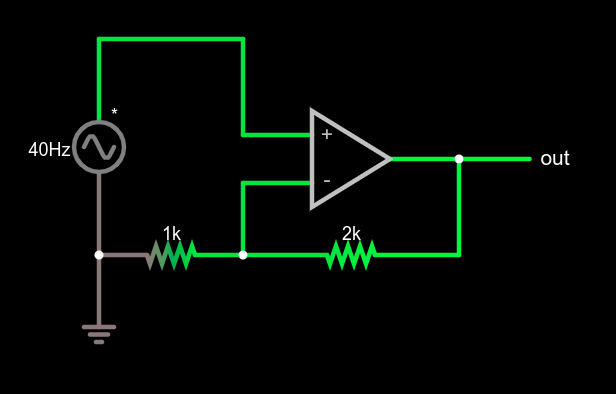
Non-inverting amplifier example
This type of configuration is called a non-inverting amplifier because, unlike an inverting amplifier, an increase in the input voltage causes an increase in the output voltage and a decrease in input causes the output to follow.
Note that the feedback voltage divider isn’t drawn like a divider, but that’s just moving symbols on paper. It is still a voltage divider just like in the earlier example. Can you figure the voltage gain of the stage? The voltage divider ratio is 1:3 and, sure enough, a 5V peak on input turns into a 15V peak on the output, so the gain is 3. Try changing the divider to different ratios.
What’s Next?
While it isn’t mathematically rigorous, thinking of the op amp as a machine that makes its inputs equal is surprisingly effective. It certainly made the analysis of these simple circuits, the comparator, the buffer amplifier, and a general non-inverting amplifier simple.
There are, of course, many other types of amplifiers, as well as other reasons to use op amps such as oscillators, filters, and other even more exotic circuits. We’ll talk about some of them next time and the idea of a virtual ground, which is another helpful analysis rule of thumb.