We’ve all been victims of bad memes on the Internet, but they’re not all just bad jokes gone wrong. Some are simply bad as a result of being copies-of-copies, as each reposter adds another layer of compression to an already lossy image format like JPEG. Compression can certainly be a benefit in areas like images and videos, but [Michal] had a bit of a fever dream imagining this process applied to text. Rather than let the idea escape, he built the Lossifizer to add JPEG-like compression to text.
JPEG compression uses a system similar to the fast Fourier transform (FFT) called the discrete cosine transform (DCT) to reduce the amount of data in an image by essentially removing some frequency information. The data lost is often not noticeable to the human eye, at least until it gets out of hand. [Michal]’s system performs the same transform on text instead, with a slider to control the “amount of JPEG” in the output text. The code for this script uses a “perceptual” character map, clustering similarly-looking and similarly-sounding characters next to each other, resembling “leet speak” from days of yore, although at high enough compression this quickly gets out of hand.
One of the quirks that [Michal] discovered is that certain AI chat bots have a much less difficult time interpreting this JPEG-ified text than a human probably would have, which provides a bit of insight into how some of these algorithms might be functioning under the hood. For some more insight into how JPEG actually works on images, we posted about a deep dive into the image format a while back.
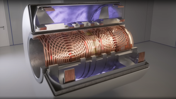
Of all the high-tech medical gadgets we read about often, the Magnetic Resonance Imaging (MRI) machine is possibly the most mysterious of all. The ability to peer inside a living body, in a minimally invasive manner whilst differentiating tissue types, in near real-time was the stuff of science fiction not too many years ago. Now it’s commonplace. But how does the machine actually work? Real Engineering on YouTube presents the Insane Engineering of MRI Machines to help us along this learning curve, at least in a little way.
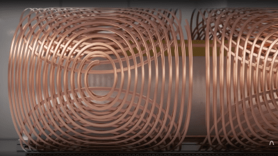
Both types of gradient coil are stacked around the subject inside the main field coil
The basic principle of operation is to align the spin ‘axis’ of all the subject’s hydrogen nuclei using an enormous magnetic field produced by a liquid-helium-cooled superconducting electromagnet. The spins are then perturbed with a carefully tuned radio frequency pulse delivered via a large drive coil.
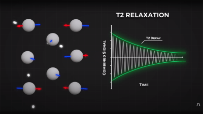
After a short time, the spins revert back to align with the magnetic field, remitting a radio pulse at the same frequency. Every single hydrogen nucleus (just a proton!) responds at roughly the same time, with the combined signal being detected by the receive coil (often the same physical coil as the driver.)
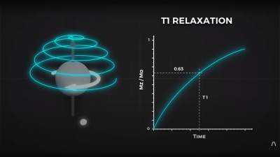
Time taken for the perturbed spin to return to magnetic alignment
There are two main issues to solve. Obviously, the whole body section is ‘transmitting’ this radio signal all in one big pulse, so how do you identify the different areas of 3D space (i.e. the different body structures) and how do you differentiate (referred to as contrast) different tissue types, such as determine if something is bone or fat?
By looking at the decay envelope of the return pulse, two separate measures with different periods can be determined; T1, the spin relaxation period, and T2, the total spin relaxation period. The first one is a measure of how long it takes the spin to realign, and the second measures the total period needed for all the individual interactions between different atoms in the subject to settle down. The values of T1 and T2 are programmed into the machine to adjust the pulse rate and observation time to favor the detection of one or the other effect, effectively selecting the type of tissue to be resolved.
Time taken for the relative phasing inside a tissue locality to settle down to the same average spin alignment
The second issue is more complex. Spatial resolution is achieved by first selecting a plane to virtually slice the body into a 2D image. Because the frequency of the RF pulse needed to knock the proton spin out of alignment is dependent upon the magnetic field strength, overlaying a second magnetic field via a gradient coil allows the local magnetic field to be tuned along the axis of the machine and with a corresponding tweak to the RF frequency an entire body slice can be selected.
All RF emissions from the subject emanate from just the selected slice reducing the 3D resolution problem to a 2D problem. Finally, a similar trick is applied orthogonally, with another set of gradient coils that adjust the relative phase of the spins of stripes of atoms through the slice. This enables the use of a 2D inverse Fourier transform of multiple phase and frequency combinations to image the slice from every angle, and a 2D image of the subject can then be reconstructed and sent to the display computer for the operator to observe.
[Stanislaw Pusep] has gifted us with the Pianolizer project – an easy-to-use toolkit for music exploration and visualization, an audio spectrum analyzer helping you turn sounds into piano notes. You can run his toolkit on a variety of different devices, from Raspberry Pi and PCs, to any browser-equipped device including smartphones, and use its note output however your heart desires. To show off his toolkit in action, he set it up on a Raspberry Pi, with Python code taking the note data and sending color information to the LED strip, displaying the notes in real time as he plays them on a MIDI keyboard! He also created a browser version that you can use with a microphone input or an audio file of your choosing, so you only need to open a webpage to play with this toolkit’s capabilities.
He took time to make sure you can build your projects with this toolkit’s help, providing usage instructions with command-line and Python examples, and even shared all the code used in the making of the demonstration video. Thanks to everything that he’s shared, now you can add piano note recognition to any project of yours! Pianolizer is a self-contained library implemented in JavaScript and C++ (which in turn compiles into WebAssembly), and the examples show how it can be used from Python or some other language.
[Stanislaw] also documented the principles behind the code, explaining how the note recognition does its magic in simple terms, yet giving many insights. We are used to Fast Fourier Transform (FFT) being our go-to approach for spectral analysis, aka, recognizing different frequencies in a stream of data. However, a general-purpose FFT algorithm is not as good for musical notes, since intervals between note frequencies become wider as frequency increases, and you need to do more work to distinguish the notes. In this toolkit, he used a Sliding Discrete Fourier Transform (SDFT) algorithm, and explains to us how he derived the parameters for it from musical note frequencies. In the end of the documentation, he also gives you a lot of useful references if you would like to explore this topic further!
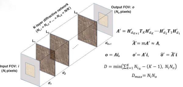
Linear transforms — like a Fourier transform — are a key math tool in engineering and science. A team from UCLA recently published a paper describing how they used deep learning techniques to design an all-optical solution for arbitrary linear transforms. The technique doesn’t use any conventional processing elements and, instead, relies on diffractive surfaces. They also describe a “data free” design approach that does not rely on deep learning.
There is obvious appeal to using light to compute transforms. The computation occurs at the speed of light and in a highly parallel fashion. The final system will have multiple diffractive surfaces to compute the final result.
Oftentimes in computing, we start doing a thing, and we’re glad we’re doing it. But then we realise, it would be much nicer if we could do it much faster. [Ricardo de Azambuja] was in just such a situation when working with the Raspberry Pi Zero, and realised that there were some techniques that could drastically speed up Fast Fourier Transforms (FFT) on the platform. Thus, he got to work.
The trick is using the Raspberry Pi Zero’s GPU to handle the FFTs instead of the CPU itself. This netted Ricardo a 7x speed upgrade for 1-dimensional FFTs, and a 2x speed upgrade for 2-dimensional operations.
The idea was cribbed from work we featured many years ago, which provided a similar speed up to the very first Raspberry Pi. Given the Pi Zero uses the same SoC as the original Raspberry Pi but at a higher clock rate, this makes perfect sense. However, in this case, [Ricardo] implemented the code in Python instead of C as suits his use case.
[Ricardo] uses the code with his Maple Syrup Pi Camera project, which pairs a Coral USB machine learning accelerator with a Pi Zero and a camera to achieve tasks such as automatic licence plate recognition or facemask detection. Fun!
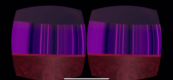
One of the hard things about electronics is that you can’t really see the working parts without some sort of tool. If you work on car engines, fashion swords, or sculpt clay, you can see with your unaided eye what’s going on. Electronic components are just abstract pieces and the real action requires a meter or oscilloscope to understand. Maybe that’s what [José] was thinking of when he built a-radio. This “humble experiment” pipes a scan from a software-defined radio into VR goggles, which can be as simple as a smartphone and some cardboard glasses.
The resulting image shows you what the radio spectrum looks like. Granted, so will a spectrum analyzer, but perhaps the immersion will provide a different kind of insight into radio frequency analysis.
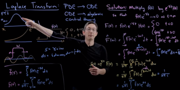
Most people who deal with electronics have heard of the Fourier transform. That mathematical process makes it possible for computers to analyze sound, video, and it also offers critical math insights for tasks ranging from pattern matching to frequency synthesis. The Laplace transform is less familiar, even though it is a generalization of the Fourier transform. [Steve Bruntun] has a good explanation of the math behind the Laplace transform in a recent video that you can see below.
There are many applications for the Laplace transform, including transforming types of differential equations. This comes up often in electronics where you have time-varying components like inductors and capacitors. Instead of having to solve a differential equation, you can perform a Laplace, solve using common algebra, and then do a reverse transform to get the right answer. This is similar to how logarithms can take a harder problem — multiplication — and change it into a simpler addition problem, but on a much larger scale.