Simulating High-Side Bootstrap Circuits With LTSpice

May 13, 2025 by Dave Rowntree 14 Comments

LTSpice is a tool that every electronics nerd should have at least a basic knowledge of. Those of us who work professionally in the analog and power worlds rely heavily on the validity of our simulations. It’s one of the basic skills taught at college, and essential to truly understand how a circuit behaves. [Mano] has quite a collection of videos about the tool, and here is a great video explanation of how a bootstrap circuit works, enabling a high-side driver to work in the context of driving a simple buck converter. However, before understanding what a bootstrap is, we need to talk a little theory.

Bootstrap circuits are very common when NMOS (or NPN) devices are used on the high side of a switching circuit, such as a half-bridge (and by extension, a full bridge) used to drive a motor or pump current into a power supply.

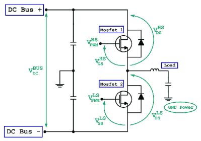
A simple half-bridge driving illustrates the high-side NMOS driving problem.

From a simplistic viewpoint, due to the apparent symmetry, you’d want to have an NMOS device at the bottom and expect a PMOS device to be at the top. However, PMOS and PNP devices are weaker, rarer and more expensive than NMOS, which is all down to the device physics; simply put, the hole mobility in silicon and most other semiconductors is much lower than the electron mobility, which results in much less current. Hence, NMOS and NPN are predominant in power circuits.

As some will be aware, to drive a high-side switching transistor, such as an NPN bipolar or an NMOS device, the source end will not be at ground, but will be tied to the switching node, which for a power supply is the output voltage. You need a way to drive the gate voltage in excess of the source or emitter end by at least the threshold voltage. This is necessary to get the device to fully turn on, to give the lowest resistance, and to cause the least power dissipation. But how do you get from the logic-level PWM control waveform to what the gate needs to switch correctly?

The answer is to use a so-called bootstrap capacitor. The idea is simple enough: during one half of the driving waveform, the capacitor is charged to some fixed voltage with respect to ground, since one end of the capacitor will be grounded periodically. On the other half cycle, the previously grounded end, jumps up to the output voltage (the source end of the high side transistor) which boosts the other side of the capacitor in excess of the source (because it got charged already) providing a temporary high-voltage floating supply than can be used to drive the high-side gate, and reliably switch on the transistor. [Mano] explains it much better in a practical scenario in the video below, but now you get the why and how of the technique.

We see videos about LTSpice quite a bit, like this excellent YouTube resource by [FesZ] for starters.

Continue reading “Simulating High-Side Bootstrap Circuits With LTSpice” →

Hacking Flux Paths: The Surprising Magnetic Bypass

February 21, 2025 by Heidi Ulrich 6 Comments

If you think shorting a transformer’s winding means big sparks and fried wires: think again. In this educational video, titled The Magnetic Bypass, [Sam Ben-Yaakov] flips this assumption. By cleverly tweaking a reluctance-based magnetic circuit, this hack channels flux in a way that breaks the usual rules. Using a simple free leg and a switched winding, the setup ensures that shorting the output doesn’t spike the current. For anyone who is obsessed with magnetic circuits or who just loves unexpected engineering quirks, this one is worth a closer look.

So, what’s going on under the hood? The trick lies in flux redistribution. In a typical transformer, shorting an auxiliary winding invites a surge of current. Here, most of the flux detours through a lower-reluctance path: the magnetic bypass. This reduces flux in the auxiliary leg, leaving voltage and current surprisingly low. [Sam]’s simulations in LTspice back it up: 10 V in yields a modest 6 mV out when shorted. It’s like telling flux where to go, but without complex electronics. It is a potential stepping stone for safer high-voltage applications, thanks to its inherent current-limiting nature.

The original video walks through the theory, circuit equivalences, and LTspice tests. Enjoy!

Continue reading “Hacking Flux Paths: The Surprising Magnetic Bypass” →

Modeling Home Heating Systems With Circuit Simulation Software

July 1, 2024 by Bryan Cockfield 6 Comments

Electricity flow is generally invisible, silent, and not something that most humans want to touch, so understanding how charge moves around can be fairly unintuitive at first. There are plenty of analogies to help understand its behavior, such as imagining a circuit as a pipe of water, with pressure standing in for voltage and flow standing in for current. But you can flip this idea in reverse and use electric circuits to model other complex phenomena instead. [Oxx], for example, is using circuit theory to model his home’s heating systems.

To build his model, he’s using LTSpice, a free circuit simulation program. Using voltage to model temperature and current to model heat flow, he’s set up a model for his home to compare the behavior of a heat pump and a propane furnace. A switch model already in LTSpice with built-in hysteresis takes the place of the thermostat. Using temperature data for a single day in January [Oxx] can see how each of his two heating systems might behave, and the model for the heat pump is incredibly close to how the heat pump behaved in real life.

The model includes all kinds of data about the system, including the coefficient of performance of the heat pump and its backup electric resistive heater, and the model is fairly accurate at predicting behavior. Of course, it takes a good bit of work to set up the parameters for all of the components since our homes and heating systems won’t be included in LTSpice by default, but it does show how powerful an electric circuit analog can be when building models of other systems. If you’ve never used this program before, we’ve featured a few guides to getting started that you can take a look at.

Thanks to [Jarvis] for the tip!

Continue reading “Modeling Home Heating Systems With Circuit Simulation Software” →

QSPICE Picks Up Where LTSpice Left Us

August 25, 2023 by Dave Rowntree 24 Comments

[Mike Engelhardt] is a name that should be very familiar to the hardcore electronics nerd. [Mike] is the developer responsible for LTSpice, which is quite likely the most widely used spice-compatible simulator in the free software domain. When you move away from digital electronics and the comfort of software with its helpful IDEs and toolchains, and dip a wary toe into the murky grey waters of analog or power electronics, LTSpice is your best friend. And, like all best friends, it’s a bit quirky, but it always has your back. Sadly, LTSpice development seems to have stalled some years ago, but luckily for us [Mike] has been busy on the successor, QSpice, under the watchful eye of Qorvo.

It does look in its early stages, but from a useability point of view, it’s much improved over LTSpice. Performance is excellent (based on this scribe’s limited testing while mobile.) Gone (thankfully!) is the uncommon verb-noun usage paradigm — replaced with a more usual cut-n-paste flow. Visually it still kind of looks like LTspice in places, but nicer with a clear and uncluttered design that gets straight to the point. Internally, the simulation engine has improved in speed and accuracy, as well as adding native support for modern semiconductor types, such as wide bandgap materials like SiC. Noted is that this updated software has a particular emphasis on power integrity and noise analysis, which are sticky problems that have a big impact on modern high-power systems.

Continue reading “QSPICE Picks Up Where LTSpice Left Us” →

Practical Inductors In LTSpice

July 18, 2023 by Al Williams 8 Comments

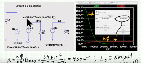
LTSpice and the underlying Spice engine does a great job of simulating ideal components. But it is also capable — if you know how — of handling models of real-world devices. Inductors, for example, are one of the most imperfect components. Their constituent wire has resistance, and there is parasitic capacitance between the windings. If there is a core, it also will have many imperfections and losses. [Sam Ben-Yaakov] has a lecture about modeling real inductors in LTSpice, and he covers how you can capture some of these imperfections in the video below.

There is a bit of math in the presentation, but we liked that it relates back to datasheets for actual components. Being able to understand what the parameters on a datasheet mean is crucial, and if you ever wondered what some of these entries mean, you’ll get a lot from this video.

The main feature of the model is the flux equation. The tanh (hyperbolic tangent) function is similar to the curve you want for the flux equation, so it plays a major part. Of course, there are other parts of the inductor you may have to model, too, but this is one of the most difficult parts.

You can also model transformers using LTSpice. You can also create custom components.

Continue reading “Practical Inductors In LTSpice” →

Freq Out With LTSpice

July 3, 2023 by Al Williams 4 Comments

We always enjoy [FesZ’s] videos, and his latest about FREQ function in LTSpice is no exception. In fact, LTSpice doesn’t document it, but it is part of the underlying Spice system. So, of course, you can figure it out or just watch the video below. The FREQ keyword allows you to change component attributes in a frequency-depended way.

Of course, capacitors and inductors are frequency dependent by design. But the FREQ technique allows you to adjust things like voltage sources or resistance in arbitrary ways. By default, you must specify the frequency response data in decibels, which isn’t always convenient. However, [FesZ] shows you how to use other methods to express them using modifiers to the command.

Continue reading “Freq Out With LTSpice” →

IBIS Models Explained

March 26, 2023 by Al Williams 2 Comments

If you’ve worked with circuit simulation, you may have run into IBIS models. The acronym is input/output buffer information, and while you can do a lot without having to deal with IBIS, knowing about it can help you have a successful simulation.

IBIS is an industry-standard format that uses ASCII text to describe voltage versus current and voltage versus time about some device’s digital input and output pins. This allows precise simulation without revealing the device’s internals, which is important to some vendors. The first post of this two-part series talks about what IBIS is and how it got started. The second part explains creating and using LTSpice to create your own IBIS models. It also covers why you might want to do that.

Of course, if you don’t care about revealing the internals of a device, you could just create a Spice simulation. However, many tools will accept both models, so it is useful to know how to produce either kind of model. In fact, to create an IBIS model, you’ll want to use a Spice model to generate the data for the IBIS model, so it is a good bet you’ll have both, even if you choose to only publish the IBIS models.

If you need a refresher on Spice, we have a series. If you prefer using something different, try Micro-Cap 12, which was commercial, but went free a few years ago.