Doesn’t the Z-axis on 3D-printers seem a little – underused? I mean, all it does is creep up a fraction of a millimeter as the printer works through each slice. It would be nice if it could work with the other two axes and actually do something interesting. Which is exactly what’s happening in the nonplanar 3D-printing methods being explored at the University of Hamburg. Printing proceeds normally up until the end, when some modifications to Slic3r allow smooth toolpaths to fill in the stairsteps and produce a smooth(er) finish. It obviously won’t work for all prints or printers, but it’s nice to see the Z-axis finally pulling its weight.
If you want to know how something breaks, best to talk to someone who looks inside broken stuff for a living. [Roger Cicala] from LensRentals.com spends a lot of time doing just that, and he has come to some interesting conclusions about how electronics gear breaks. For his money, the prime culprit in camera and lens breakdowns is side-mounted buttons and jacks. The reason why is obvious once you think about it: components mounted perpendicular to the force needed to operate them are subject to a torque. That’s a problem when the only thing holding the component to the board is a few SMD solder pads. He covers some other interesting failure modes, too, and the whole article is worth a read to learn how not to design a robust product.
In the seemingly neverending quest to build the world’s worst Bitcoin mining rig, behold the 8BitCoin. It uses the 6502 processor in an Apple ][ to perform the necessary hashes, and it took a bit of doing to port the 32-bit SHA256 routines to an 8-bit platform. But therein lies the hack. But what about performance? Something something heat death of the universe…
Contributing Editor [Tom Nardi] dropped a tip about a new online magazine for people like us. Dubbed Paged Out!, the online quarterly ‘zine is a collection of contributed stories from hackers, programmers, retrocomputing buffs, and pretty much anyone with something to say. Each article is one page and is formatted however the author wants to, which leads to some interesting layouts. You can check out the current issue here; they’re still looking for a bunch of articles for the next issue, so maybe consider writing up something for them – after you put it on Hackaday.io, of course.
Tipline stalwart [Qes] let us know about an interesting development in semiconductor manufacturing. Rather than concentrating on making transistors smaller, a team at Tufts University is making transistors from threads. Not threads of silicon, or quantum threads, or threads as a metaphor for something small and high-tech. Actual threads, like for sewing. Of course, there’s plenty more involved, like carbon nanotubes — hey, it was either that or graphene, right? — gold wires, and something called an ionogel that holds the whole thing together in a blob of electrolyte. The idea is to remove all rigid components and make truly flexible circuits. The possibilities for wearable sensors could be endless.
And finally, here’s a neat design for an ergonomic utility knife. It’s from our friend [Eric Strebel], an industrial designer who has been teaching us all a lot about his field through his YouTube channel. This knife is a minimalist affair, designed for those times when you need more than an X-Acto but a full utility knife is prohibitively bulky. [Eric’s] design is a simple 3D-printed clamshell that holds a standard utility knife blade firmly while providing good grip thanks to thoughtfully positioned finger depressions. We always get a kick out of watching [Eric] design little widgets like these; there’s a lot to learn from watching his design process.
Thanks to [JRD] and [mgsouth] for tips.