An Op-Amp From The Ground Up

January 30, 2021 by Jenny List 49 Comments

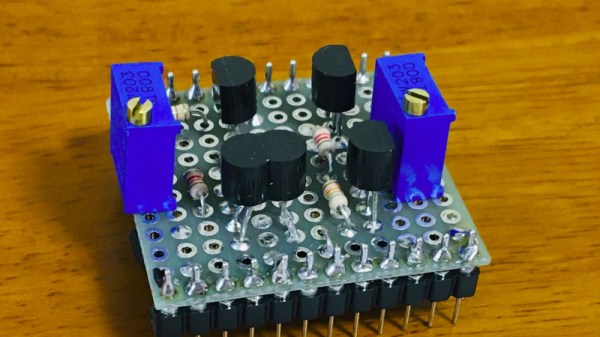
If we had to pick one part to crown as the universal component in the world of analogue electronics, it would have to be the operational amplifier. The humble op-amp can be configured into so many circuit building blocks that it has become an indispensable tool for designers. It’s tempting to treat an op-amp as a triangular black box in a circuit diagram, but understanding its operation gives an insight into analogue electronics that’s worth having. [Mitsuru Yamada]’s homemade op-amp using discrete components is thus a project of interest, implementing as it does a complete simple op-amp with five transistors.

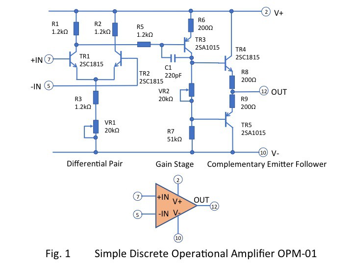Looking at the circuit diagram it follows the classic op-amp with a long-tailed pair of NPN transistors driving a PNP gain stage and finally a complimentary emitter follower as an output buffer. It incorporates the feedback capacitor that would have been an external component on early op-amp chips, and it has a couple of variable resistors to adjust the bias. Keen eyed readers will notice its flaws such as inevitably mismatched transistors and the lack of a current mirror in the long-tailed pair, but using those to find fault in a circuit built for learning is beside the point. He demonstrated it in use, and even goes as far as to show it running an audio power amplifier driving a small speaker.

For the dedicated student of op-amps, may we suggest further reading as we examine the first integrated circuit op-amp?

Homebrew Slide Rule Gets Back To Mathematical Basics

November 11, 2020 by Dan Maloney 49 Comments

In the grand scheme of things, it really wasn’t all that long ago that a slide rule was part of an engineer’s every day equipment. Long before electronic calculators came along, a couple of sticks of wood inscribed with accurate scales was all it took to do everything from simple multiplication to logarithms and trig functions.

While finding a slide rule these days isn’t impossible, it’s still not exactly easy, and buying one off the shelf isn’t as fun or as instructive as building one yourself. [JavierL90]’s slide rule build started, ironically enough, on the computer, with a Python program designed to graphically plot the various scales needed for the fixed sections of the slide rules (the “stators”) and the moving bit (the “slide”). His first throught was to laser-engrave the scales, but the route of printing them onto self-adhesive vinyl stock proved to be easier.

With the scale squared away, work turned to the mechanism itself. He chose walnut for the wood, aluminum for the brackets, and a 3D-printed frame holding a thin acrylic window for the sliding cursor. The woodworking is simple but well-done, as is the metalwork. We especially like the method used to create the cursor line — a simple line scored into the acrylic with a razor, which was then filled with red inks. The assembled slide rule is a thing of beauty, looking for all the world like a commercial model, especially when decked out with its custom faux leather carry case.

We have to admit that the use of a slide rule is a life skill that passed us by, but seeing this puts us in the mood for another try. We might have to start really, really simple and work up from there.

Eye-Catching And Crumb-Suspending

September 10, 2020 by Brian McEvoy 5 Comments

Printed circuit boards used to be green or tan, and invariably hidden. Now, they can be artful, structural, and like electronic convention badges, they are the entire project. In this vein, we find Open LEV, a horseshoe-shaped desktop bauble bristling with analog circuitry supporting an acoustic levitator. [John Loefler] is a mechanical engineer manager at a college 3D printing lab in Florida, so of course, he needs to have the nerdiest stuff on his workspace. Instead of resorting to a microcontroller, he filled out a parts list with analog components. We have to assume that the rest of his time went into making his PCB show-room ready. Parts of the silkscreen layer are functional too. If you look closely at where the ultrasonic transducers (silver cylinders) connect, there are depth gauges to aid positioning. Now that’s clever.

Continue reading “Eye-Catching And Crumb-Suspending” →

An Analog IC Design Book Draft

August 31, 2020 by Al Williams 21 Comments

[Jean-Francois Debroux] spent 35 years designing analog ASICs. He’s started a book and while it isn’t finished — indeed he says it may never be — the 180 pages he posted on LinkedIn are a pretty good read.

The 46 sections are well organized, although some are placeholders. There are sections on design flow and the technical aspects of design. Examples range from a square root circuit to a sigma-delta modulator, although some of them are not complete yet. There are also sections on math, physics, common electronics, materials, and tools.

Continue reading “An Analog IC Design Book Draft” →

Analog Noise Generator, Fighter Of Other Noises

July 6, 2020 by Donald Papp 11 Comments

A chaotic drone of meaningless sound to lull the human brain out of its usual drive to latch on to patterns can at times be a welcome thing. A nonsense background din — like an old television tuned to a dead channel — can help drown out distractions and other invading sounds when earplugs aren’t enough. As [mitxela] explains, this can be done with an MP3 file of white noise, and that is a solution that works perfectly well for most practical purposes. However he found himself wanting a more refined hardware noise generator with analog controls to fine tune the output, and so the Rumbler was born.

The Rumbler isn’t just a white noise generator. White noise has a flat spectrum, but the noise from the Rumbler is closer to Red or Brownian Noise. The different colors of noise have specific definitions, but the Rumbler’s output is really just white noise that has been put through some low pass filters to create an output closer to a nice background rumble that sounds pleasant, whereas white noise is more like flat static.

Why bother with doing this? Mainly because building things is fun, but there is also the idea that this is better at blocking out nuisance sounds from neighboring human activities. By the time distant music (or television, or talking, or shouting) has trickled through walls and into one’s eardrums, the higher frequencies have been much more strongly attenuated than the lower frequencies. This is why one can easily hear the bass from a nearby party’s music, but the lyrics don’t survive the trip through walls and windows nearly as well. The noise from the Rumbler is simply a better fit to those more durable lower frequencies.

[Mitxela]’s writeup has quite a few useful tips on analog design and prototyping, so give it a read even if you’re not planning to make your own analog noise box. Want to hear the Rumbler for yourself? There’s an embedded audio sample near the bottom of the page, so go check it out.

For a truly modern application of white noise, check out the cone of silence for snooping smart speakers.

An Open Hardware Modem For The Modern Era

June 9, 2020 by Tom Nardi 39 Comments

Readers of a certain age will no doubt remember the external modems that used to sit next to their computers, with the madly flashing LEDs and cacophony of familiar squeals announcing your impending connection to a realm of infinite possibilities. By comparison, connecting to the Internet these days is about as exciting as flicking on the kitchen light. Perhaps even less so.

But while we don’t use them to connect our devices to the Internet anymore, that doesn’t mean the analog modem is completely without its use. The OpenModem by [Mark Qvist] is an open hardware and software audio frequency-shift keying (AFSK) modem that recalls some of the charm (and connection speeds) of those early devices.

It’s intended primarily for packet radio communications, and as such is designed to tie into a radio’s Push-to-Talk functionality with a standard 3.5 mm jack connector. Support for AES-128 encryption means it will take a bit more than an RTL-SDR to eavesdrop on your communications. Though if you’re really worried about others listening in, the project page says you could even use the OpenModem over a wired connection as you would have in the old days.

If you just want a simple and reliable way to get a secure AFSK communication link going, the OpenModem looks like it would be a great choice. But more than that, it offers a compelling platform for learning and experimentation. The hardware is compatible with the Arduino IDE, so you can even write your own firmware should you want to spin up your own take on this classic communications device.

The OpenModem is the evolution of the MicroModem that [Mark] developed years ago, and it’s clear that the project has come a long way since then. Of course, if you’re more about the look than the underlying technology, you could always just put a WiFi access point into the case of an old analog modem.

[Thanks to Boofdas for the tip.]

Receive Analog Video Radio Signals From Scratch

May 31, 2020 by Bryan Cockfield 6 Comments

If you’ve been on the RTL-SDR forums lately you may have seen that a lot of work has been going into the DragonOS software. This is a software-defined radio group that has seen a lot of effort put into a purpose-built Debian-based Linux distribution that can do a lot of SDR out of the box. The latest and most exciting project coming from them involves a method for using the software to receive and demodulate analog video.

[Aaron]’s video (linked below) demonstrates using a particular piece of software called SigDigger to analyze an incoming analog video stream from a drone using a HackRF. (Of course any incoming analog signal could be used, it doesn’t need to be a drone.) The software shows the various active frequency ranges, allows a user to narrow in on one and then start demodulating it. While it has to be dialed in just right to get anything that doesn’t look like snow, [Aaron] is able to get recognizable results in just a few minutes.

Getting something like this to work completely in software is an impressive feat, especially considering that all of the software used here is free. Granted, this wouldn’t be as easy for a digital signal like most TV stations broadcast, but there’s still a lot of fun to be had. In case you missed the release of DragonOS, we covered it a few weeks ago and it’s only gotten better since then, with this project just as one example.

Continue reading “Receive Analog Video Radio Signals From Scratch” →